Sampling with Open Paths

Figure 5.1: Illustration of a permutation of closed and open paths showing imaginary time $T$ vs. one spatial dimension $x$. In the left graph, a permutation of three closed paths, each with a different lines style, is displayed. $t_p$ denotes the slice where the relabelling of the particle indices takes place. The fermion determinant is always positive. On the right, a two particle permutation involving an open paths with the open end at $\frac{\beta}{2}$ is shown. Slice for which the fermion determinant has to be negative, are indicated.

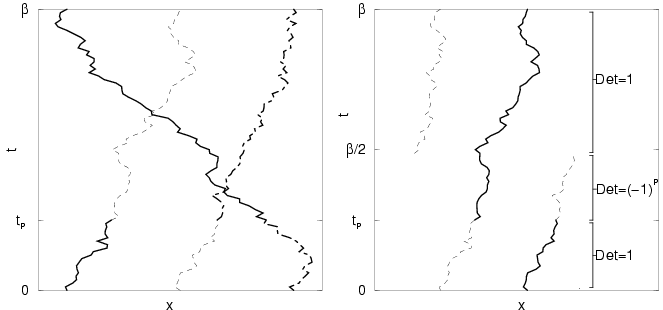
In this section, the multilevel sampling procedure from sections 2.5.3 and 2.6.9 will be extended to the sampling with open paths for Bosons and distinguishable particles. Fermions will be discussed in section 5.2. A picture of an open path is shown in Fig. 5.1. We chose to put the open ends at time slice $\frac{\beta}{2}$ because we will apply the double reference method from section 2.6.4 to fermionic systems. For distinguishable particles, the open path is a single polymer that interacts with the other particles. The contributions to the action are calculated in the same way as is done for closed paths except for the diagonal pair action in the time slice containing the open ends. There, each open end contributes with the weight $\frac{1}{2}$, which can be understood from Eq. 2.25.

Without interactions, the distribution of the open ends is by definition given by the free particle density matrix in Eq. 2.11. This equation will be used in the free particle sampling method for the generation of new path sections that contain the open ends. For closed paths, one samples the new positions from a Gaussian distribution centered at the midpoint between the slice above and below (Eq. 2.63) because of the two spring terms in the free particle action. The open ends are only connected in one direction in imaginary time. Therefore, the free particle sampling distribution for open ends being connected to ${\bf r}_{i+1}$ or ${\bf r}_{i-1}$ reads,

$$T({\bf r}_i) = (4 \pi \lambda \tau)^{-D/2} \exp \left \{ -... ...bf r}_i-{\bf r}_{i \pm 1})^2}{4 \lambda \tau} \right \} \quad.$$ (210)

For Bosons and Fermions, one also needs to sample the permutation space, which can be done as for closed paths described in section 2.5.4. The open paths can then form long chains consisting of several particles. Those correspond to off-diagonal long-range order. In $^4$He, they lead to the condensate fraction of atoms with precisely zero momentum as shown by Ceperley (1995).