Sampling Procedure

The sampling procedure used in the MC simulations consists of several steps, which will be briefly described here,

1. Select the time slices to be modified ( $i \ldots i+2^k$) either at random or by making random steps with an upper limit.

2. Build a permutation table containing up to 3 particle permutations using the probability similar to Eq. 2.69
   

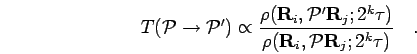   $$T({\mathcal{P}}\to {\mathcal{P}}') \propto \frac{ \rho({\bf... ... { \rho({\bf R}_i,{\mathcal{P}}{\bf R}_{j}; 2^k \tau) } \quad.$$ (115)

   
   
   This can be considered the zeroth step in the multilevel sampling procedure. Dividing out the current permutation term has the advantage that it lead to 100% acceptance for free particles in the following first slice sampling step. In the case of fermions and close paths, permutations of a even number of particles do not enter the table since they will inevitably lead to a violation of the nodes.

3. Determine the new midpoints given by 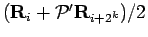$({\bf R}_i+{\mathcal{P}}'{\bf R}_{i+2^k})/2$, sample the new coordinates from Eq. 2.64 and accept with probability,
   

   $$A(s_k \to s'_k) = \mbox{min} \left\{ \,1 \, , \, T({\mathca... ...k(s'_k) } { T_k(s_k \to s'_k) \, \pi_k(s_k) } \right\} \quad.$$ (116)

   
   
   We use only the diagonal part of the pair action at this level. Note that for high levels where $\sqrt{2^k \lambda \tau}$ is of the order of the box size, corrections to $T_k$ need to be considered because points in the tail of the Gaussian fall out of the box and are mapped back in by the periodic boundary conditions. This leads to additional terms in the probability of sampling a particular point. If this move of rejected here or at any later stage continue at step 2 or 1.

4. Continue the bisection method based on Eq. 2.66 down to level 1. Consider the long-range as well as the off-diagonal pair action only at the last level.

5. Perform a Metropolis rejection step on the permutations by calculating the probability for the reverse move,
   

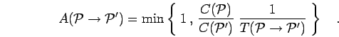   $$A({\mathcal{P}}\to {\mathcal{P}}') = \mbox{min} \left\{ \;1 ... ...frac{1}{T({\mathcal{P}}\to {\mathcal{P}}')} \; \right\} \quad.$$ (117)

   
   
   The factor $\left[ T({\mathcal{P}}\to {\mathcal{P}}') \right]^{-1}$ cancels with the extra term in Eq. 2.107.

6. Check the nodal surfaces in each slice, verify that $\rho_T({\bf R}_t,{\bf R}^*;t)>0$.

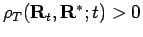7. Make a Metropolis rejection step based on the difference in the nodal action,
   

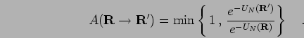   $$A({\bf R}\to {\bf R}') = \mbox{min} \left\{ \,1 \, , \, \frac{ e^{-U_N({\bf R}')} }{ e^{-U_N({\bf R})} } \right\} \quad.$$ (118)

   
   

8. Upon final acceptance, update all coordinates. Continue at step 1 or 2.

Some averages are calculated at every step, others less frequently e.g. only when one moves to a new section of the paths. In the MC simulation, some displacement moves are intertwined with the multilevel sampling moves described above. This completes the description for a simulation with closed paths. The modifications required for open paths are discussed in chapter 5.