Permutation Sampling

Fermi and Bose statistics require to sum over all permutations in addition to the integration in real space. Both can be combined into one MC process that samples configurations in the space of coordinates and permutations.

In Eq. 2.47, one sums paths beginning at ${\bf R}$ and going to ${\mathcal{P}}{\bf R}'$. One can also think of two sets of coordinates ${\bf R}$ and ${\bf R}'$, for which one integrates over all possible ways to link the individual particles. In this picture, the permutation of the paths can be carried out at any time slice because the permutation operator permutes with the Hamiltonian. This is what is done in the actual MC simulation. One selects a time slice denoted by $t_{\mathcal{P}}$, at which one switches from the unpermuted to the permuted coordinates. $t_{\mathcal{P}}$ can be shifted to any slice along the paths. In a permutation move, one introduces a new permutation and simultaneously regrows the paths between the fixed points ${\bf R}_i$ and ${\bf R}_{j}$ with $j=i+2^k$. The equilibrium distribution of the permutation is given by,

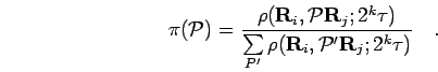$$\pi({\mathcal{P}}) = \frac{\rho({\bf R}_i,{\mathcal{P}}{\bf... ...} \rho({\bf R}_i,{\mathcal{P}}' {\bf R}_{j}; 2^k \tau)} \quad.$$ (78)

Since there are $N!$ permutations, it is advisable to put an upper limit on the step size in permutation space. Typically, one only considers changes in current permutations that involve the cyclic exchange of up to 3 or 4 particles. Since the normalization is known in Eq. 2.69 one can use the heat bath transition rule, in which a permutation ${\mathcal{P}}'$ is sampled from the neighborhood ${\mathcal{N}}({\mathcal{P}})$ of the current permutation ${\mathcal{P}}$ using their equilibrium distribution,

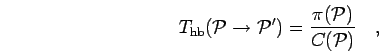$$T_{\rm hb}({\mathcal{P}}\to {\mathcal{P}}') = \frac{\pi({\mathcal{P}})}{C({\mathcal{P}})} \quad,$$ (79)

where the normalization is given by the sum over all neighboring states,

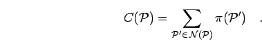$$C({\mathcal{P}}) = \sum_{{\mathcal{P}}' \in \, {\mathcal{N}}({\mathcal{P}})} \pi({\mathcal{P}}') \quad.$$ (80)

The acceptance probability follows from Eq. 2.53,

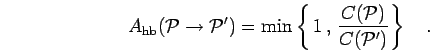$$A_{\rm hb}({\mathcal{P}}\to {\mathcal{P}}') = \mbox{min} \le... ... \frac{ C({\mathcal{P}}) }{C({\mathcal{P}}')} \right\} \quad.$$ (81)

If the neighborhoods of ${\mathcal{P}}$ and ${\mathcal{P}}'$ are equal, all moves will be accepted. In the MC simulation, one uses the free particle density matrix to construct a permutation table containing all permutations in the neighborhood. Then ${\mathcal{P}}'$ is selected and accepted with the probability in Eq. 2.72, which does not exactly equal one unless the permutation table exhausts the whole space.