Metropolis Monte Carlo

Most path integral calculations work with a Metropolis rejection algorithm (Metropolis et al., 1953), in which a Markov process is constructed in order to generate a random walk through state space, $\{s_0,s_1,s_2,\ldots\}$. A transition rule $P(s\rightarrow s')$ depending on the initial state $s$ and the final state $s'$ is exploited to step from $s_i$ to $s_{i+1}$, which is chosen in such a way that the distribution of $\{s_n\}$ converges to a given distribution $\pi(s)$. If the transition rule is ergodic and fulfills the detailed balance

$$\pi(s)\,P(s\rightarrow s') = \pi(s')\,P(s'\rightarrow s),$$ (59)

then the probability distribution converges to an equilibrium state satisfying,

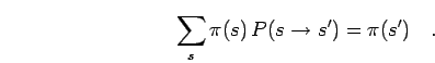$$\sum_s \pi(s)\,P(s\rightarrow s') = \pi(s') \quad.$$ (60)

The transition probability $P(s\rightarrow s')$ can be split into two parts, the sampling distribution $T(s\to s')$ that determines how the next trial state $s'$ is selected in state $s$ and the acceptance probability $A(s\to s')$ for the particular step,

$$P(s\to s') = T(s\to s') \, A(s\to s') \quad.$$ (61)

The detailed balance can be satisfied by choosing $A(s\to s')$ to be,

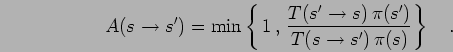$$A(s\to s') = \mbox{min} \left\{ \,1 \, , \, \frac{ T(s' \to s) \, \pi(s') }{T(s\to s') \, \pi(s) } \right\} \quad.$$ (62)

One starts the MC process at any arbitrary state $s$. Most likely this state has only a very small probability because in thermodynamic system, $\pi(s)$ is a sharply peaked function that usually spans many orders of magnitude. Therefore, it would be overrepresented in averages calculated from,

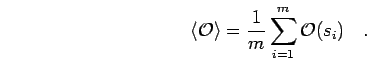$$\left< {\mathcal{O}}\right> = \frac{1}{m} \sum_{i=1}^m {\mathcal{O}}(s_i) \quad.$$ (63)

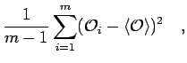
In the averages, one notices a transient behavior that eventually reaches a regime, where it fluctuates around a steady mean. From approximately that point on, one starts to collect statistics. For uncorrelated measurements, the estimator for the standard deviation $\sigma$ and the error bars $\epsilon$ can be determined from

$$\sigma_{\mathcal{O}}^2 = \frac{1}{m-1} \sum_{i=1}^m ({\mathcal{O}}_i - \left<{\mathcal{O}}\right> )^2\quad,$$ (64)

$$\epsilon_{\mathcal{O}} = \frac{\sigma_{\mathcal{O}}}{\sqrt{m}} \quad.$$ (65)

However, in most MC simulations the events are correlated because one only moves a small fraction of the particles at a time. The correlation time $\kappa$ can be shown to be estimated by

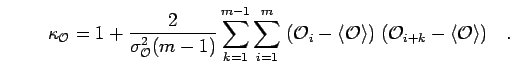$$\kappa_{\mathcal{O}}= 1 + \frac{2}{\sigma_{\mathcal{O}}^2 (m... ...>) \; ({\mathcal{O}}_{i+k}- \left<{\mathcal{O}}\right>) \quad.$$ (66)

The true statistical error considering correlations is given by

$$\epsilon_{\mathcal{O}}\; \sqrt{\kappa_{\mathcal{O}}} \quad.$$ (67)

Alternatively, it can be obtained from a blocking analysis. There, one averages over $2^m$ events ${\mathcal{O}}_i$ before calculating the error bar from Eq. 2.56. This error will grow as a function of $m$ and eventually converge when the interval $2^m$ is long enough that the averages can be considered to be statistically independent. It should be noted that there can be different reasons for correlations in MC simulations that can occur on different time scales. In certain cases, it becomes difficult to estimate the correlation time from Eq. 2.55 because of long correlations that can only be determine accurately from very long series of simulations data.

The aim of an efficient MC procedure is to decrease the error bars as rapidly as possible for given computer time. The efficiency is defined by,

$$\frac{1}{\kappa_{\mathcal{O}}\sigma_{\mathcal{O}}^2 T_s} \quad,$$ (68)

where $T_s$ is the computer time per step.

For certain applications, the sampling distribution $\pi(s)$ leads to error bars for a subset of observables that are too large. A typical example in classical MC is the pair correlation function $g(r)$ at small distances. In those cases, importance sampling can be applied. One employs an importance function $f(s)$ to generate a Markov chain according to modified distribution

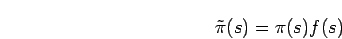$$\tilde{\pi}(s) = \pi(s) f(s)$$ (69)

rather than to $\pi(s)$. In the end, one divides it out and calculates averages from

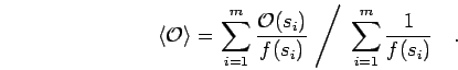$$\left< {\mathcal{O}}\right> = \left. \sum_{i=1}^{m} \frac{ {... ...(s_i)} \; \right/ \; \sum_{i=1}^{m} \frac{ 1 }{f(s_i)} \quad.$$ (70)

This method will be applied to the sampling with open paths in chapter 5. It works well as long as the modifications to the sampling distribution are not too disruptive. Otherwise, the variance $\sigma_{\mathcal{O}}$ grows or even becomes infinite. A sufficient condition for the applicability is that $\left< {\mathcal{O}}^2 \right>$ stays finite.