


Next: Permutation Sampling
Up: Monte Carlo Sampling
Previous: Single Slice Moves
Contents
Multilevel Moves
One notices that the average displacement in a single slice move is
of order
 , which means that the diffusion through
phase space goes to zero for small time steps. This is clearly an
unwanted effect in particular because one would like to have an
algorithm that is almost independent of the time step. This can be
done by introducing multi-slice moves. Instead of moving one
bead one cuts out and regrows a whole section of the path containing
, which means that the diffusion through
phase space goes to zero for small time steps. This is clearly an
unwanted effect in particular because one would like to have an
algorithm that is almost independent of the time step. This can be
done by introducing multi-slice moves. Instead of moving one
bead one cuts out and regrows a whole section of the path containing
 slices. The number
  is called the level of the move. Different
methods have been suggested to regrow the path such as Lévy
flights (Lévy, 1939) or the bisection method. The latter method will be
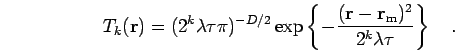
described here using free particle sampling. The distribution in
Eq. 2.63 for any level reads,
is called the level of the move. Different
methods have been suggested to regrow the path such as Lévy
flights (Lévy, 1939) or the bisection method. The latter method will be
described here using free particle sampling. The distribution in
Eq. 2.63 for any level reads,
 |
(73) |
First, one samples the bead  at slice
  from a Gaussian
distribution
from a Gaussian
distribution  centered at the midpoint of and
 . As a second step with
  , one samples the slices corresponding to
the next lower level and
, one samples the slices corresponding to
the next lower level and  using the new
  and
then keeps filling in the new coordinates until level
and
then keeps filling in the new coordinates until level  is reached and
a complete set of trial coordinates has been created. Finally, one
performs one Metropolis step on the entire move.
is reached and
a complete set of trial coordinates has been created. Finally, one
performs one Metropolis step on the entire move.
The efficiency of this method can be improved by a multilevel
Metropolis method. It rejects certain unlikely paths at an earlier
level instead of waiting until the end and then using a single metropolis
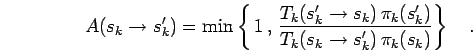
step. One starts at the highest level , samples beads
according to , and accepts with
 |
(74) |
Note that the sampling distribution as well as the probability
function  are derived from the density matrix corresponding to
the time step
are derived from the density matrix corresponding to
the time step  . If the move is rejected one starts again
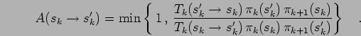
from the beginning. Otherwise, one continues at the next lower level
and samples all the midpoints according to the new
and uses a modified acceptance probability,
. If the move is rejected one starts again
from the beginning. Otherwise, one continues at the next lower level
and samples all the midpoints according to the new
and uses a modified acceptance probability,
 |
(75) |
The bisection is continued until the final level has been accepted. Only in
this case, the particle coordinates are updated. This method has the
advantage that unlikely moves are rejected early. The algorithm as a
whole satisfies detailed balance because it is fulfilled on each level,
 |
(76) |
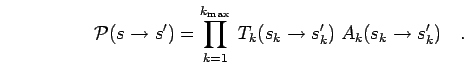
The total transition probability for the move being accepted at all
levels is given by the following product,
 |
(77) |
It is worth noting that one can use an approximate form of for
all levels except for the lowest. These kinds of approximation modify
only the acceptance ratios but not the MC averages. Therefore, it can
be advantageous to use a simplified action, which can be computed
faster. We often used the approximation
 ,
which means that we can re-use the diagonal part of the pair action
from the previous levels. Furthermore, the long-range as well as the
off-diagonal contributions to the action are only calculated at the
lowest level.
,
which means that we can re-use the diagonal part of the pair action
from the previous levels. Furthermore, the long-range as well as the
off-diagonal contributions to the action are only calculated at the
lowest level.
Next: Permutation Sampling
Up: Monte Carlo Sampling
Previous: Single Slice Moves
Contents
Burkhard Militzer
2003-01-15