Imaginary Time Path Integrals

The underlying principle for the introduction of path integrals in imaginary time is the product property of the density matrix stating that the low temperature density matrix can be expressed as a product of high temperature matrices. In operator notation this reads,

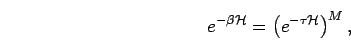$$e^{ - \beta {\mathcal{H}}} = \left( e^{ - \tau {\mathcal{H}}} \right)^M,$$ (27)

where the time step is $\tau = \beta / M$. In position space this becomes a convolution, in which one has to integrate over all intermediate time slices,

$$\rho({\bf R},{\bf R}';\beta) = \int \!\! \ldots \!\! \int {... ...bf R}_{2};\tau ) \ldots \rho({\bf R}_{M-1},{\bf R}' ;\tau ).$$ (28)

This is called a path integral in imaginary time. The expression is exact for any $M \ge 1$. In the limit $M \to \infty$, it becomes a continuous paths beginning at ${\bf R}$ and ending at ${\bf R}'$.

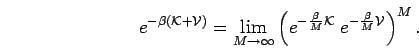
The reason for using a path integral is in the limit of high temperature, the density matrix can be calculated. Usually the Hamiltonian can be split in a kinetic and in a potential part, ${\mathcal{H}}=\mathcal{K}+\mathcal{V}$ and the density matrix can expressed using the following operator identity (Raedt and Raedt, 1983),

$$e^{-\tau(\mathcal{K}+\mathcal{V})} = e^{-\tau \mathcal{K}} e... ...mathcal{V}} e^{-\tau^2 C_2} e^{-\tau^3 C_3} +O(\tau^4) \quad,$$ (29)

where

$$C_2 = \left[ A,B\right] /2 \quad,\quad\quad\quad\quad\quad\quad\quad$$ (30)

and

$$C_3 = \left[ \left[ B,A\right],A+2B\right] /6\quad\quad\quad \quad.$$ (31)

In the limit of $\tau \to 0$, one can neglect the commutators, which are of higher order in $\tau$. This is known as the primitive approximation,

$$e^{-\tau(\mathcal{K}+\mathcal{V})} \approx e^{-\tau \mathcal{K}} e^{-\tau \mathcal{V}} \quad.$$ (32)

It states that in the limit of $M \to \infty$, the density matrix can be written as product of a potential and kinetic density matrix. This has been shown by Trotter (1959),

$$e^{-\beta (\mathcal{K}+\mathcal{V})} = \lim_{M \to \infty} ... ...M} \mathcal{K}} \; e^{-\frac{\beta}{M} \mathcal{V}} \right)^M.$$ (33)

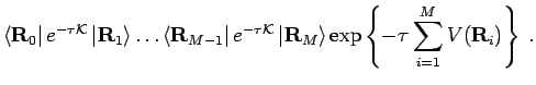
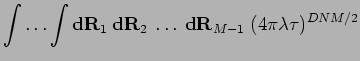
The density matrix for a system of $N$ particles in the primitive approximation is given by,

$$\rho({\bf R}_0,{\bf R}_M, \beta) = \int\ldots\int {\bf d}{\bf R}_{1} \:{\bf d}{\bf R}_{2} \:\ldots\: {\bf d}{\bf R}_{M-1} \; (4 \pi \lambda \tau)^{D N M /2}$$

$$\quad\times \; \mbox{exp} \left \{ -\sum_{i=1}^{M} \left[ \frac{(... ...frac{\tau}{2} \left( V({\bf R}_{i-1}) + V({\bf R}_i) \right) \right] \right \}.$$ (34)

In the path integral formalism this is written as,

$$\rho({\bf R},{\bf R}'; \beta) = \! \! \! \int \limits_{{\bf... ... } \! \! \! \! {\bf d}{\bf R}_t \;\; e^{-S[{\bf R}_t] }\quad,$$ (35)

where $S[{\bf R}_t]$ is the action of the path. Alternatively, one separates the kinetic and potential parts,

$$\rho({\bf R}_0,{\bf R}_M, \beta) = \int\ldots\int {\bf d}{\bf R}_{1} \:{\bf d}{\bf R}_{2} \:\ldots\: {\bf d}{\bf R}_{M-1} \;$$

$$\left< {\bf R}_0 \right\vert e^{-\tau\mathcal{K}} \left\vert {\bf... ...}_M \right> \mbox{exp} \left \{ -\tau \sum_{i=1}^{M} V({\bf R}_i) \right \} \;.$$

The free particle terms act like a weight over all Brownian random walks (BRW) in imaginary time $\beta$ starting at ${\bf R}_0$ and ending at ${\bf R}_M$. In the limit of $M \to \infty$, this leads to the Feynman-Kac relation

$$\rho({\bf R},{\bf R}', \beta) = \rho_0({\bf R},{\bf R}', \be... ...\int_0^\beta \! dt \; V({\bf R}(t)) } \right>_{\rm BRW} \quad.$$ (36)

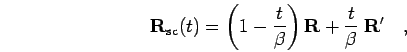
In the semi-classical approximation, one considers only the classical path,

$${\bf R}_{\rm sc}(t) = \left(1-\frac{t}{\beta}\right) {\bf R}+ \frac{t}{\beta} \; {\bf R}' \quad,$$ (37)

instead of integrating over all BRW. The resulting semi-classical density matrix reads,

$$\rho_{\rm sc}({\bf R},{\bf R}', \beta) = \rho_0({\bf R},{\bf... ... \; e^{- \int_0^\beta \! dt \; V({\bf R}_{\rm sc}(t)) } \quad.$$ (38)

Already, the primitive approximation is a sufficient basis for a path integral Monte Carlo simulation. However, the required number of time slices to reach accurate results would be enormous. The following sections, we discuss methods to derive a more accurate high temperature density matrix in order to reduce the number of slices to a computationally feasible level. A pair action will be derived, which contains the exact solution of the two particle problem. This means only one time slice is required for a simulation of two particles at any temperature. However, in many particle systems, a path integral is needed because of many-particle effects and the fermion nodes, which will be discussed in section 2.6.