Instructor:	Burkhard Militzer	GSI: tbd	tbd
	militzer@berkeley.edu	...	...
Office hours:	Tu 6-7pm	tbd	tbd

     

4 units:	Lectures:	Tu 5-6 pm	50 Birge Hall	Computer labs:	Most are on Wednesdays. For time and location
		Th 5-6 pm	50 Birge Hall		see UCB's schedule of classes.

This course offers a general introduction to computer simulations for all science majors. Participants will use the Jupyter notebooks to perform calculations, design 3D graphics, and build on existing computer programs. No prior programming experience is required. The course teaches fundamental skills for scientists and helps students with future homework. It covers data processing techniques as well standard simulations methods including Monte Carlo and molecular dynamics. The algorithms are illustrated with a variety of applications in earth and planetary science as well as astronomy.

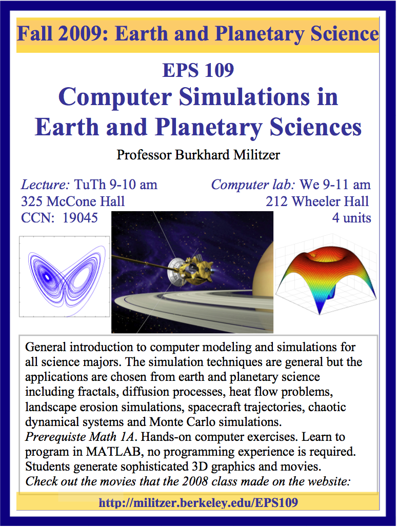
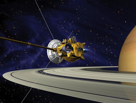
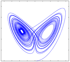
Cassini spacecraft in Saturn orbit	Choatic behavior of dynamical systems: the Lorenz attractor	Combined gravity field of sun and planet
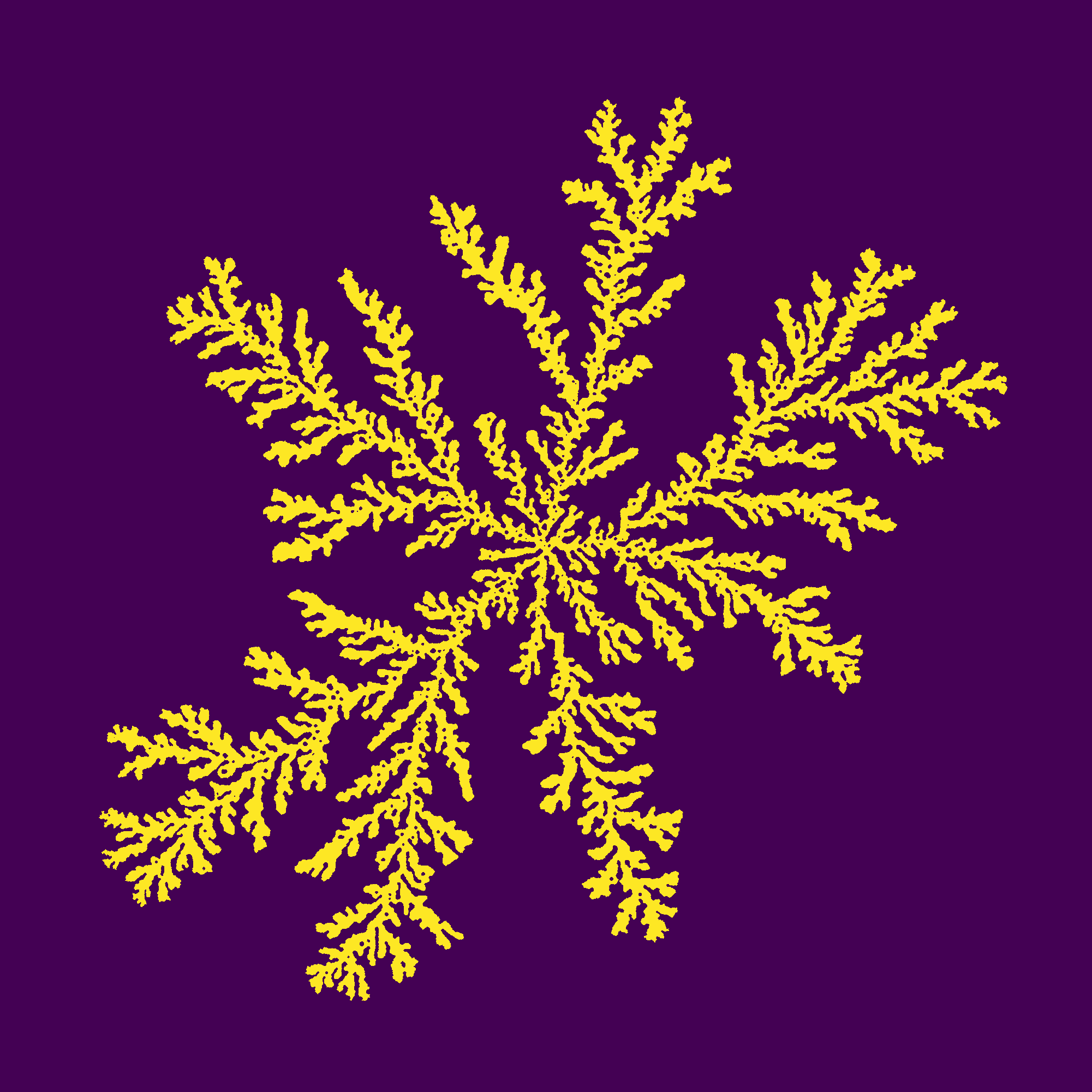
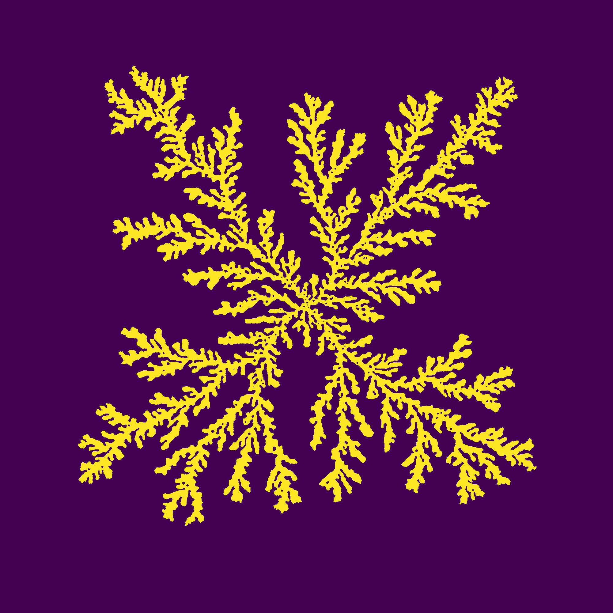
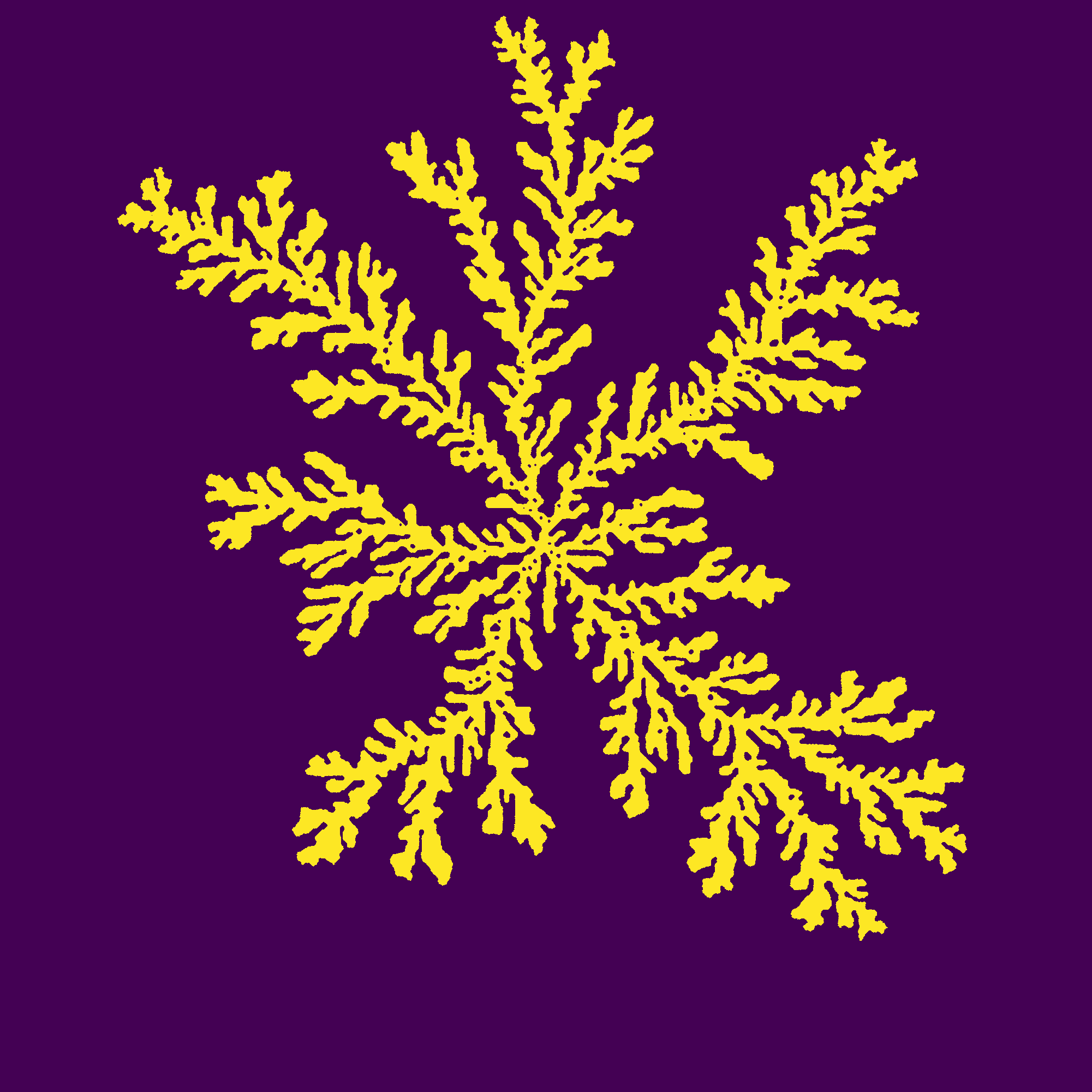
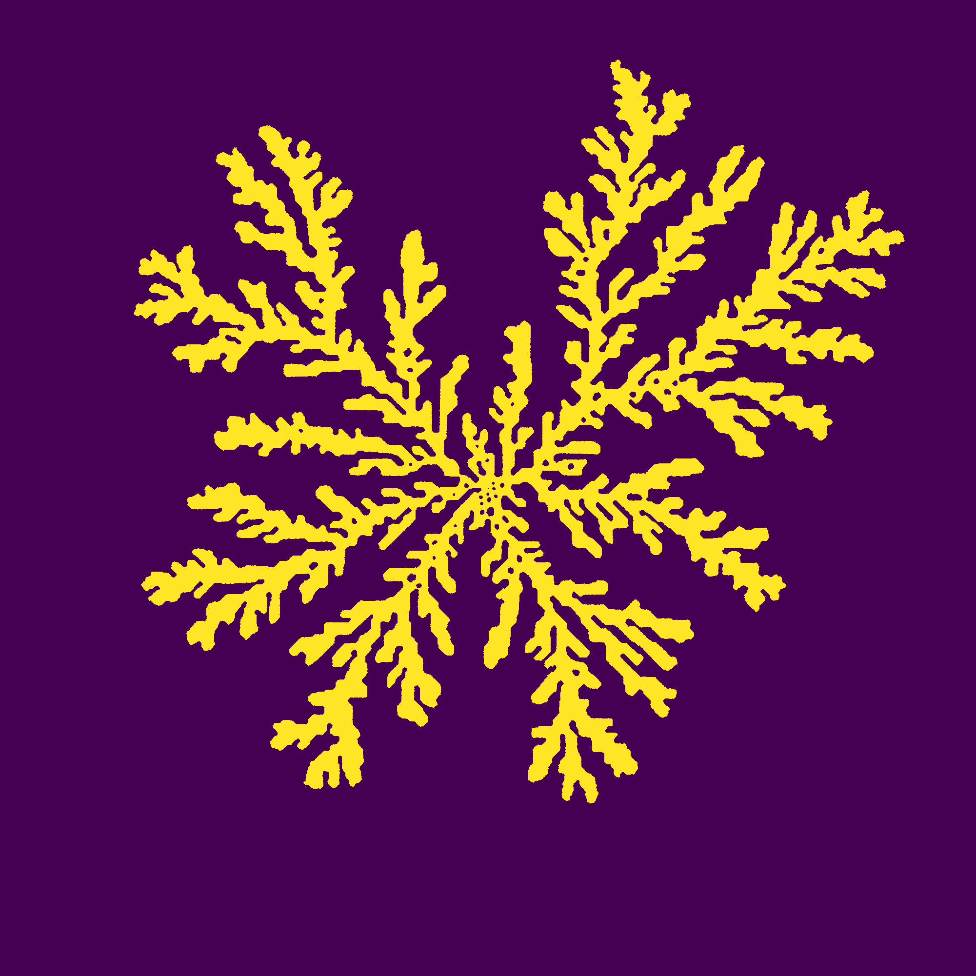
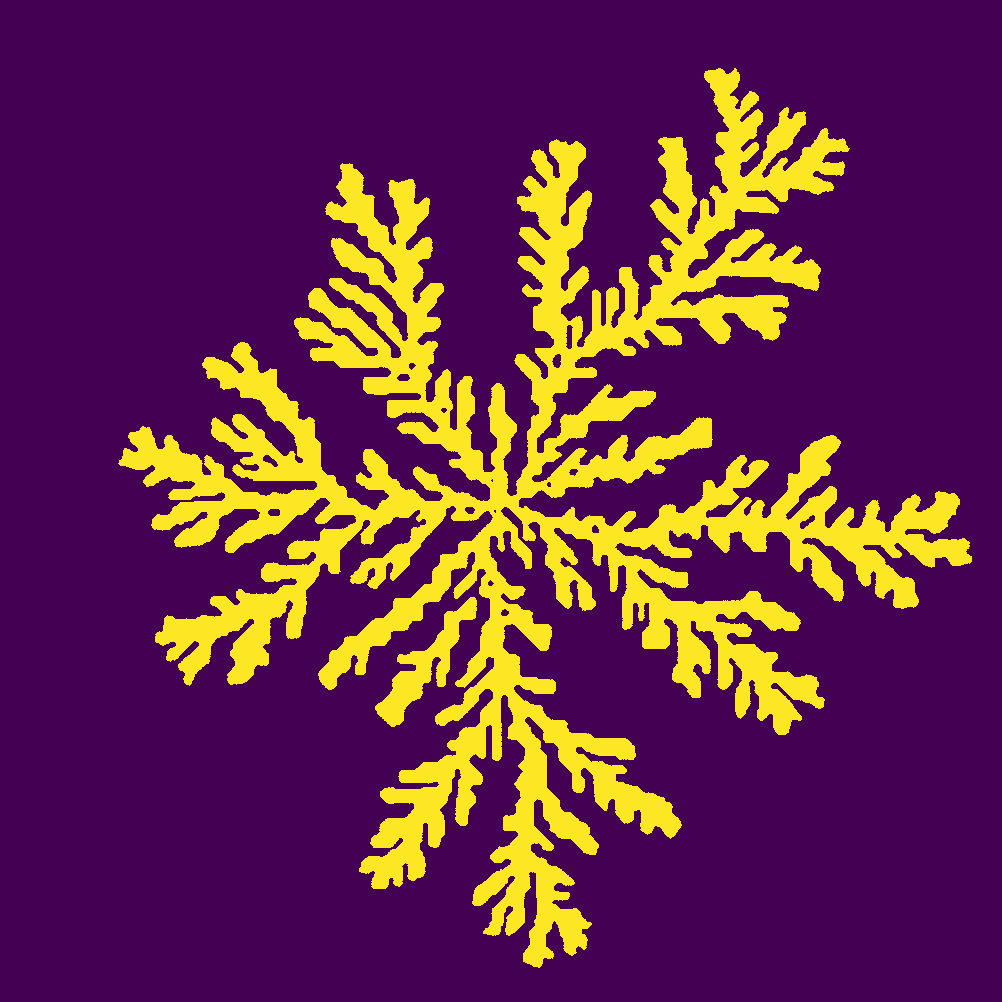
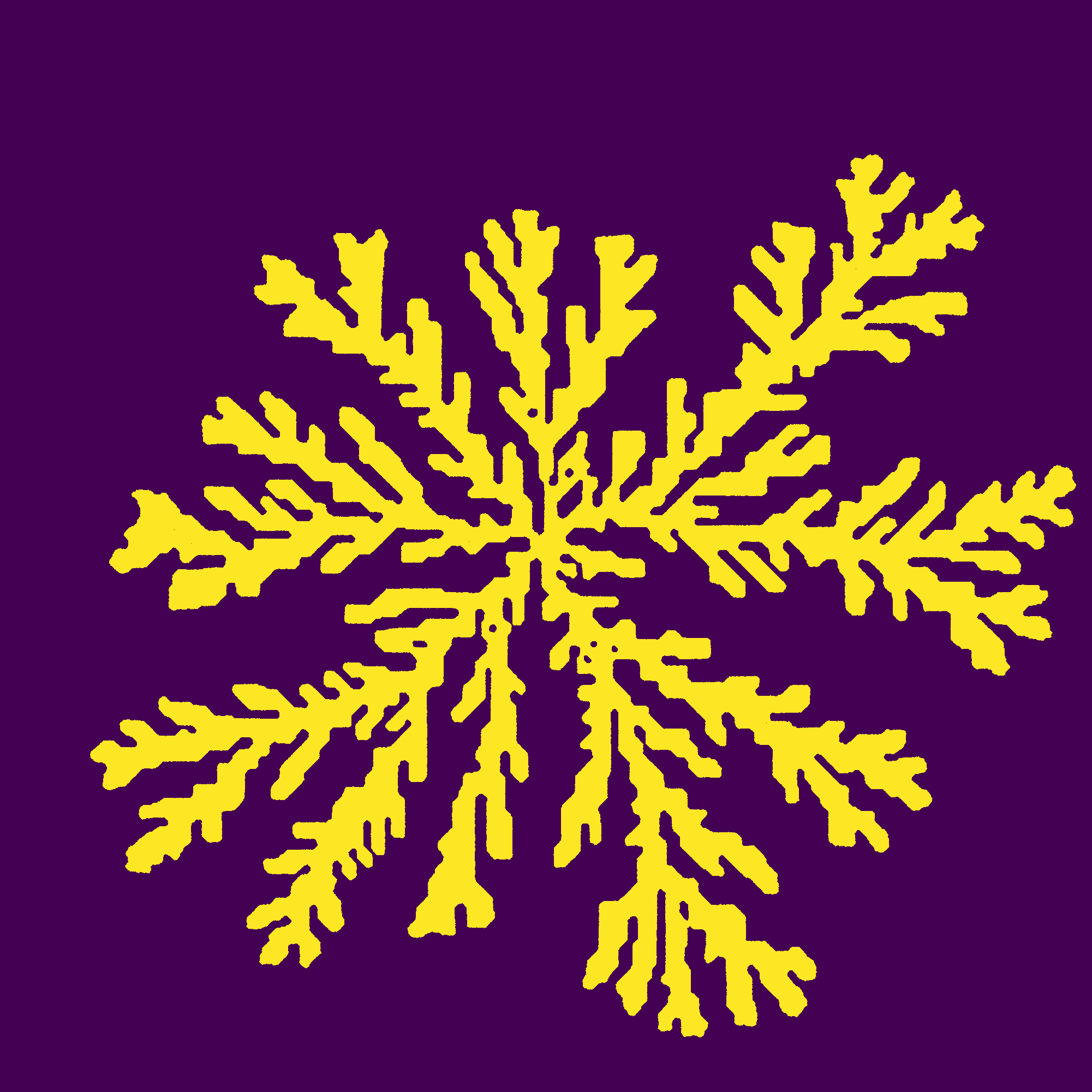
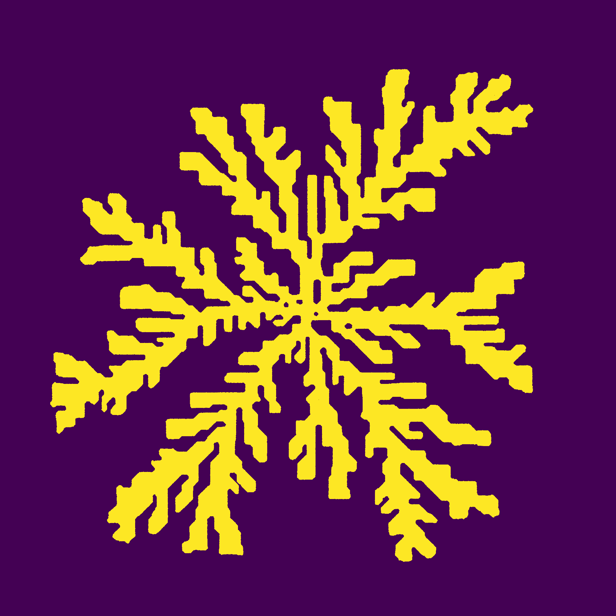
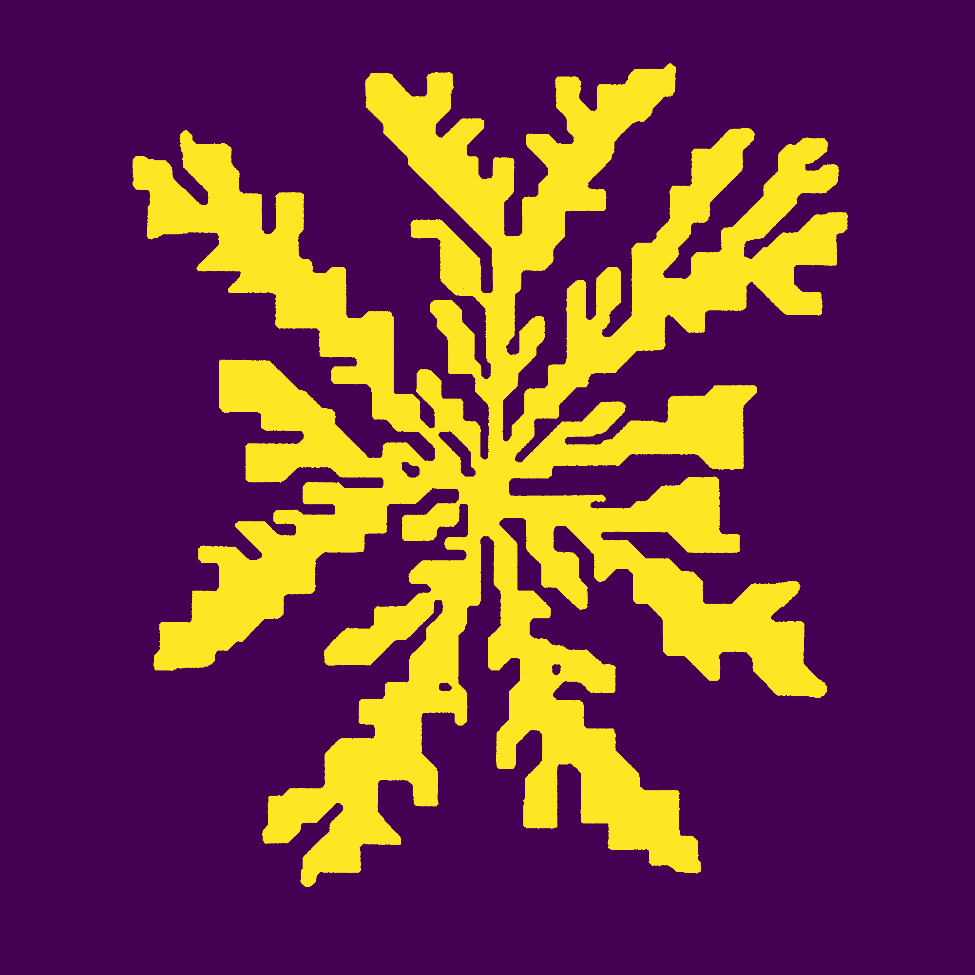
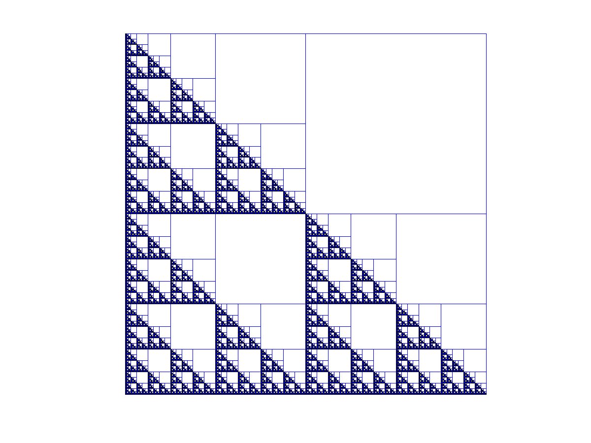
Fractal nature of ferns	Koch snowflake	Sierpinski gasket

Selected computer lab exercises and homework assignments from our 2018 Python class:

In 2018, the class switched from using Matlab to Jupyter notebooks. While there appears to be a general trend in that direction, the real motivation was the fact that all our students' Matlab codes would stop working once they left the university and their relatively inexpensive Matlab student licenses would expire. To do the following Jupyter exercises, we recommend

1) you install Anaconda on your Mac or PC.
2) Make a new directory Jupyter in home directory and place any data files like ice_core_temperature_data.txt there.
3) Start the Jupyter system from a Terminal with the commands:
        cd ~/Jupyter
        jupyter lab
4) Start a new notebook "File->New notebook" and step-by-step paste the commands for the first lab assignment Intro_to_python_05.pdf. Press SHIFT+RETURN each time.

Type of assignment	Description	Files
Lab 1	Getting to know Jupyter notebooks	Intro_to_python_05.pdf ice_core_temperature_data.txt
Homework 1	Simple calculations with Jupyter notebooks	hw01_course_intro13.pdf ice_core_CO2_data.txt
Lab 2	Pixel graphs and filling matrices	pixel_graphics12.pdf topography_180x360_grid.txt
Homework 2	Practice making a smiley	hw02_pixel_graphics_13.pdf

In this course, we generate a number of simple animations and store them as MP4 files. Here are two examples wave1d.ipynb and wave2d.ipynb that use the FFMPEG package in combination with the screen grab function. We found them more convenient than typical Python animations packages that require the user to supply the graphics for an arbitrary frame index.

Computer lab exercises and homework assignments from our 2016 Matlab class:

Type of assignment	Description	Files
Lab 1	Getting to know Matlab: vectors and matrices	lab01_Matlab_intro.pdf
Homework 1	Getting to know Matlab: loops and plots	hw01_Matlab_intro.pdf
Lab 2	Pixel graphics and ocean volume	lab02_pixel_and_ocean_volume.pdf example.m topography_18x18_grid.txt topography_180x360_grid.txt
Homework 2	Pixel graphics and ocean volume	hw02_pixel_and_ocean_volume.pdf
Lab and homework 3	Logistic map	lab_hw03_logistic_map.pdf run_sin2.m sin2.m
Lab 4	Mandelbrot set	lab04_Mandelbrot.pdf mandelbrot.m
Homework 4	San Andeas fault, Mandelbrot and Newton fractals	hw04_San_Andreas_fault_and_Mandelbrot.pdf san_andreas.m SA_fault.txt CA_coast_line.txt plate.txt CA_coast_line_no_islands.txt
Lab and homework 5	Diffusion limited aggregation	lab05_DLA.pdf hw05_DLA.pdf diffusion_limited_aggregation2D_lab01.m
Lab and homework 6	Stationary state of heat equation	lab06_heat.pdf hw06_heat.pdf
Lab and homework 7	Solving the 1D heat equation in real time. Cooling of a lava dike	lab07_heat_real_time.pdf hw07_cooling_lava.pdf
Lab and homework 8	Solving the 2D heat equation and animations	lab08_2D_heat.pdf hw08_2D_heat.pdf
Lab 9	Landscape evolution model	lab09_erosion.pdf erosion_lab_start.m calculate_collection_area2.m pool_check8.m
Homework 9	Erosion of a landscape you created	hw09_erosion.pdf erosion_ocean07.m calculate_collection_area2.m pool_check10.m initial_conditions_add_hill.m
Lab 10	Shallow water waves	lab10_water_waves.pdf waterwaves03.m
Homework 10	Waves over a mid-ocean ridge	hw10_water_waves04.pdf waterwave10.m
Lab and homework 11	Tadpole and horseshoe orbits	lab11_kepler.pdf hw11_tadpole_horseshoe_orbits.pdf run_kepler_ode.m kepler_ode.m
Homework 12	Image processing	hw12_image_processing.pdf HW12.zip
Lab and homework 13	Chaos in dynamical systems: Rossler attractor	lab_hw_13_roessler_attractor08.pdf

Additional examples that will be discussed in this course:

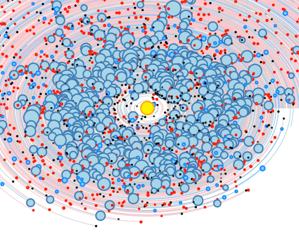
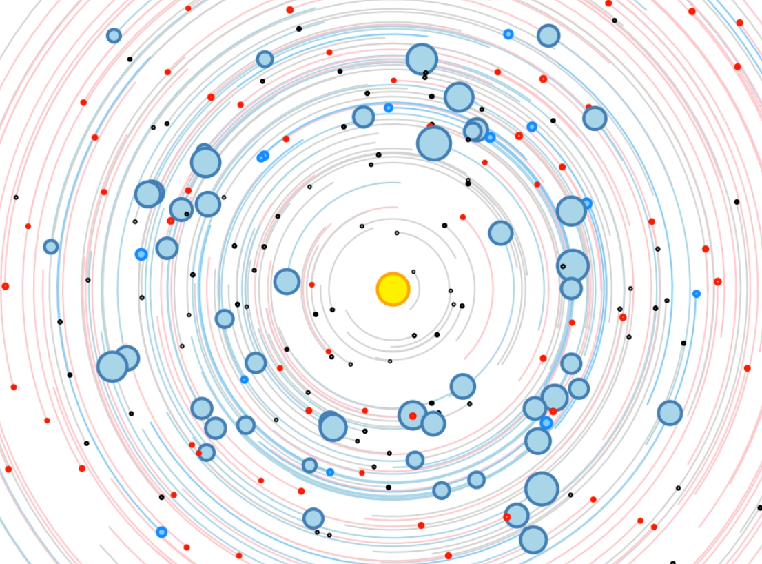
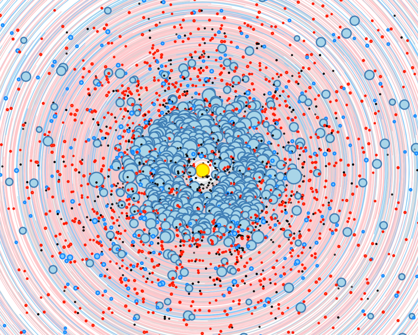
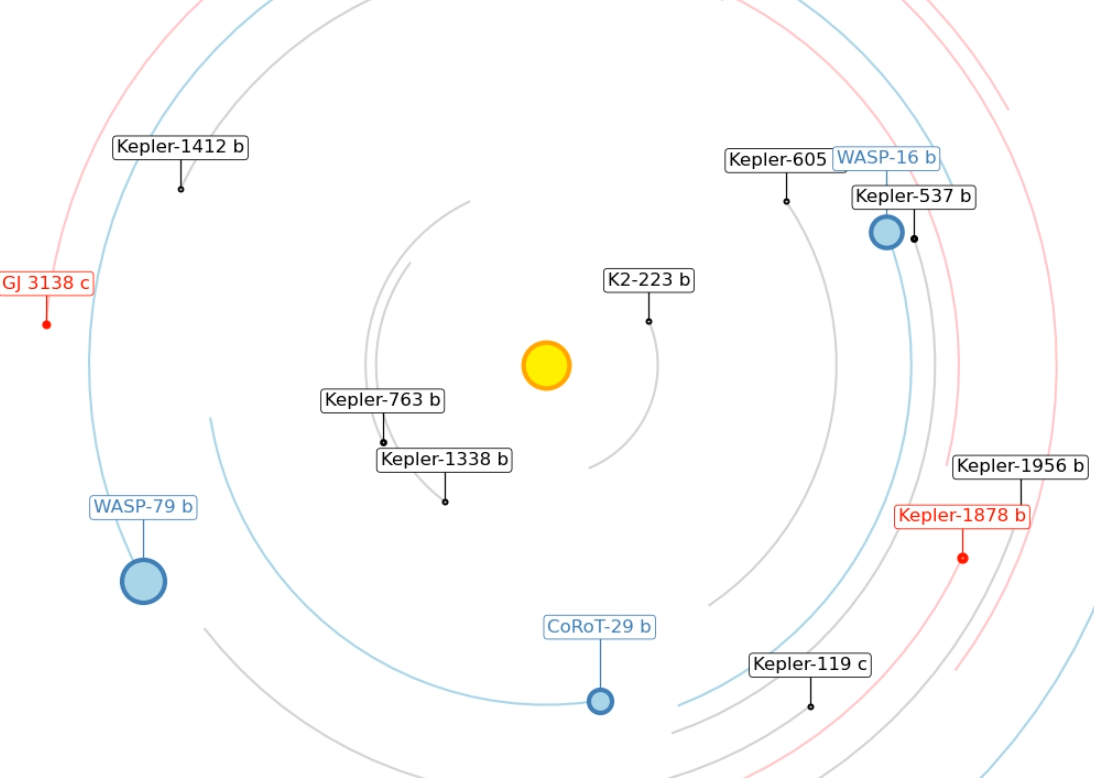
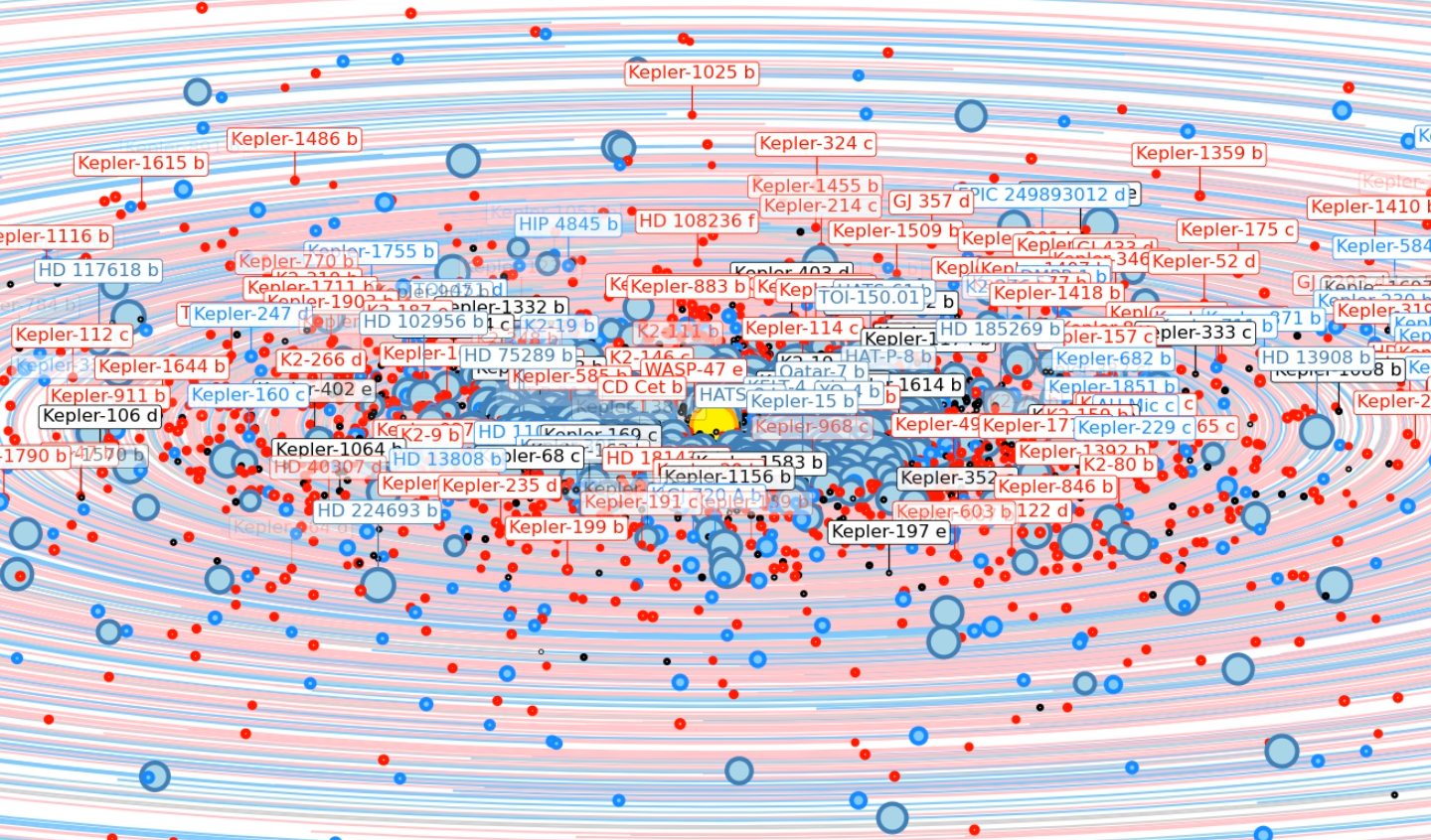
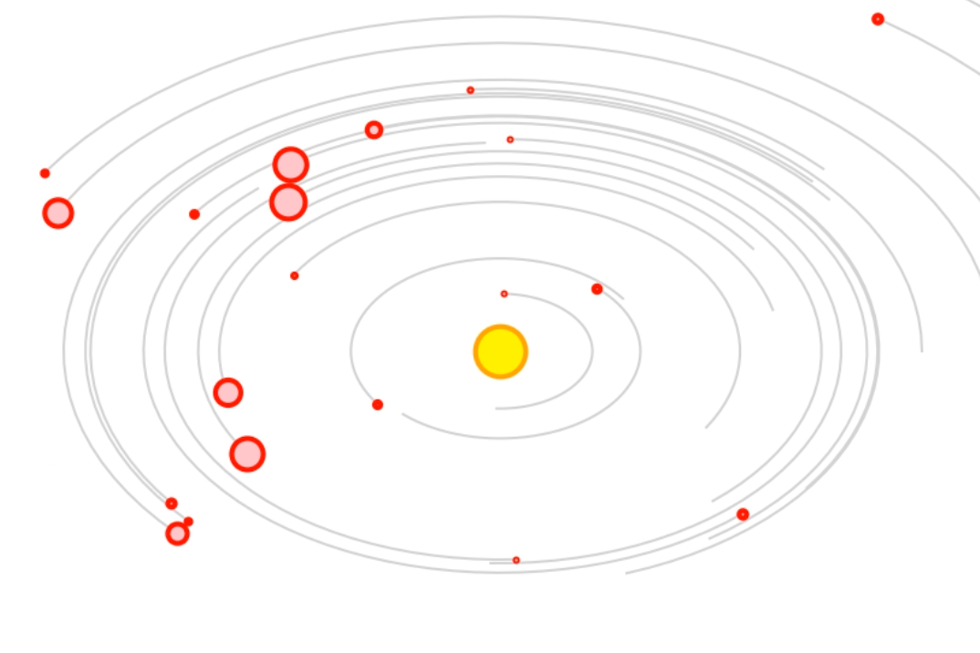
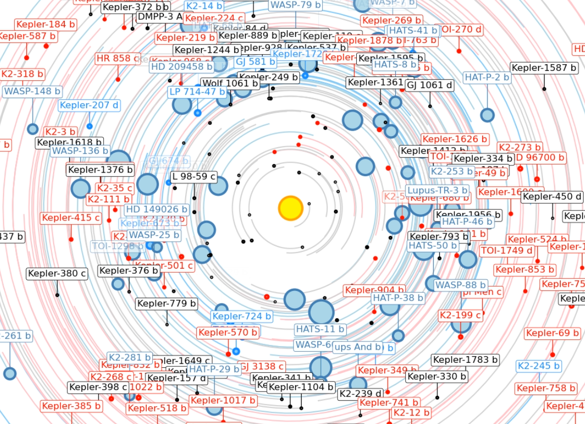
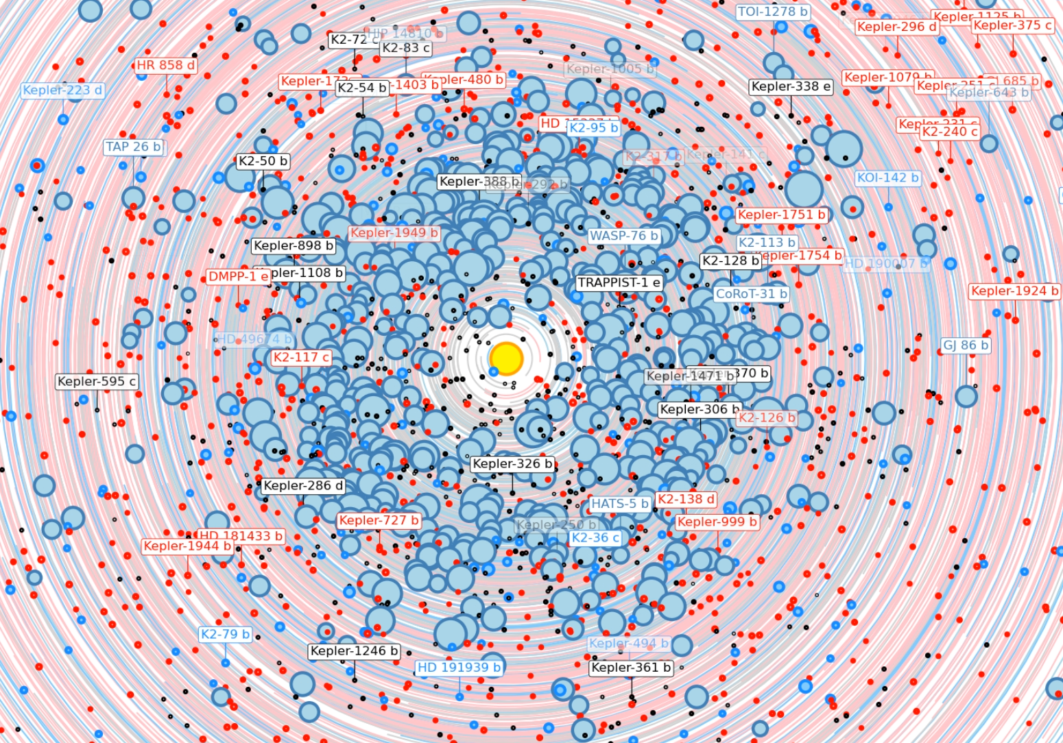
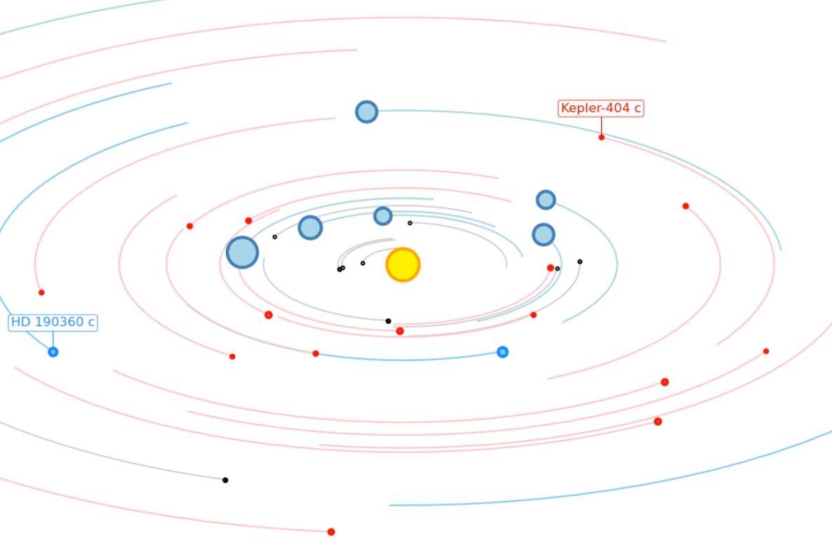
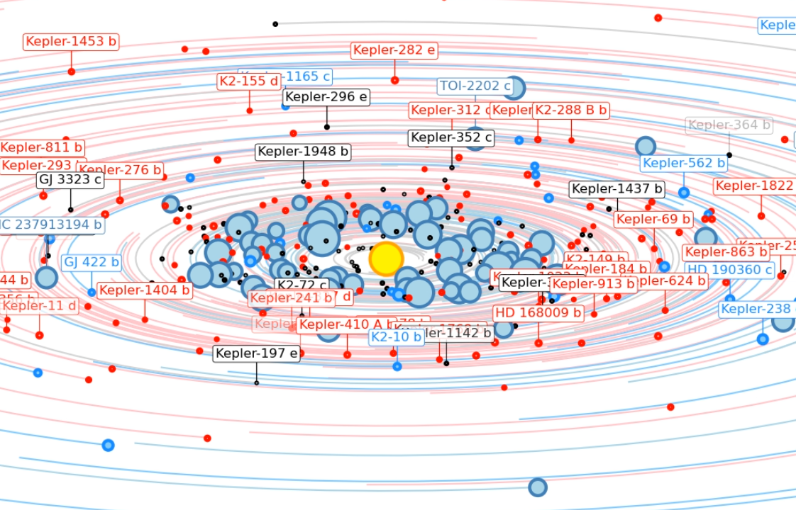
Exoplanet Orrery - Simulation of exoplanet ensembles - The orbits of the known exoplanets have been combined into a single animation. Click on any image to play the corresponding .mp4 animation. Files are between 20 MB and 1.3 GB large. If you only see a black screen, you may have to click reload to start the animation. It is best to download the file with "Save linked file as ..." and play it back with the VLC player since it does not seem to have any issues with large files.
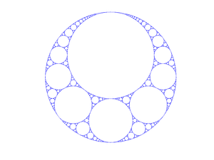
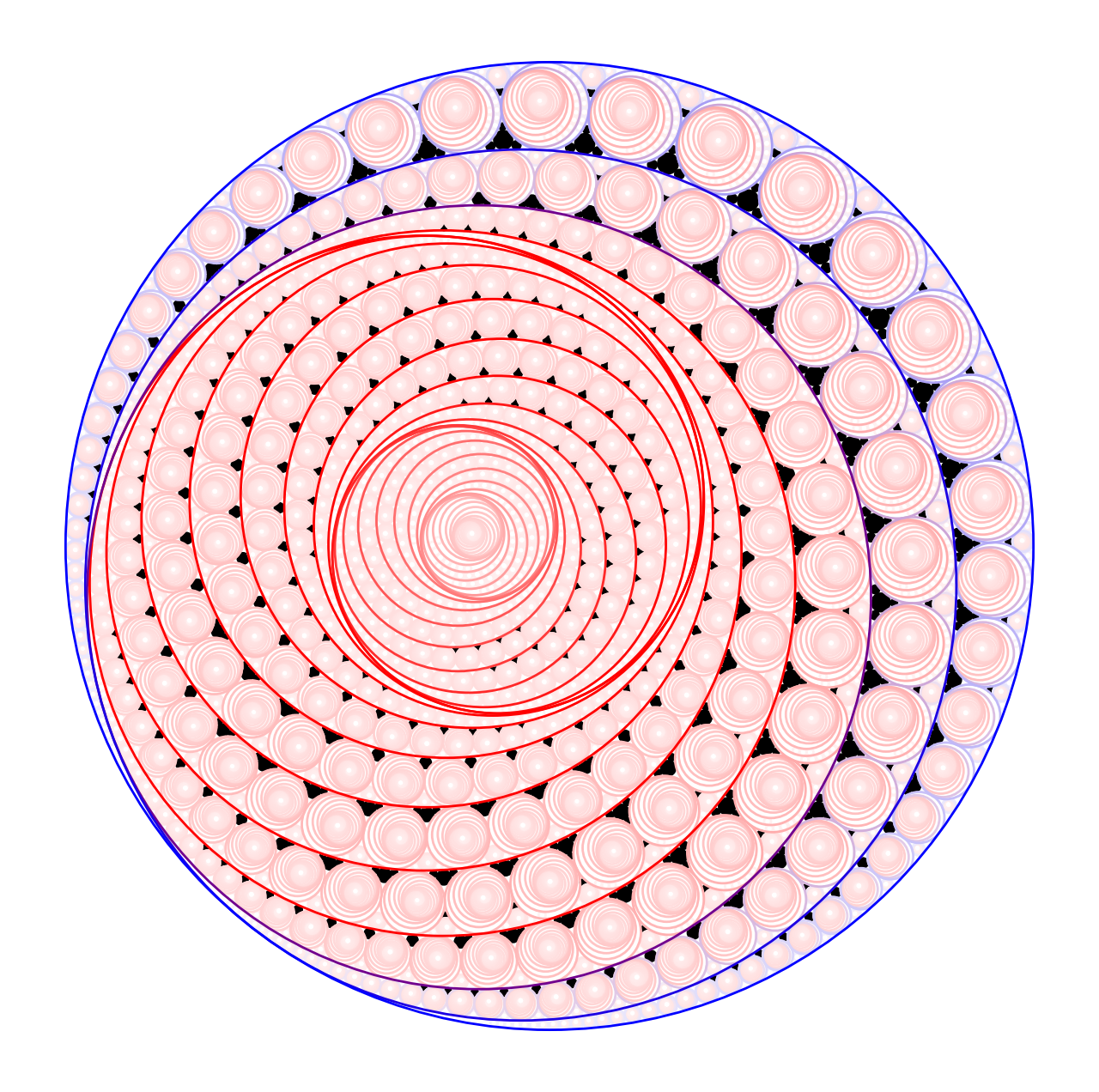
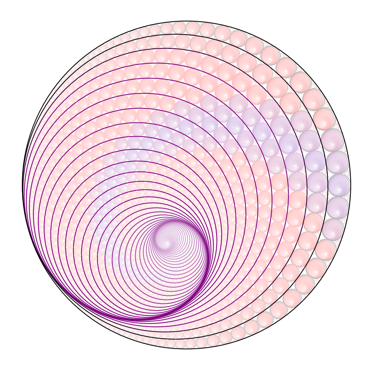
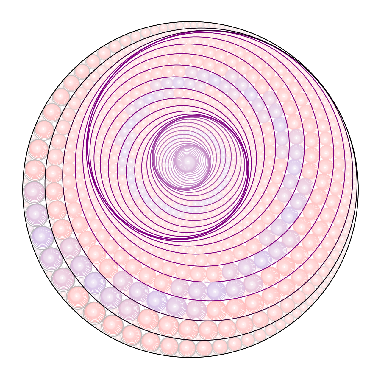
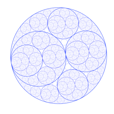
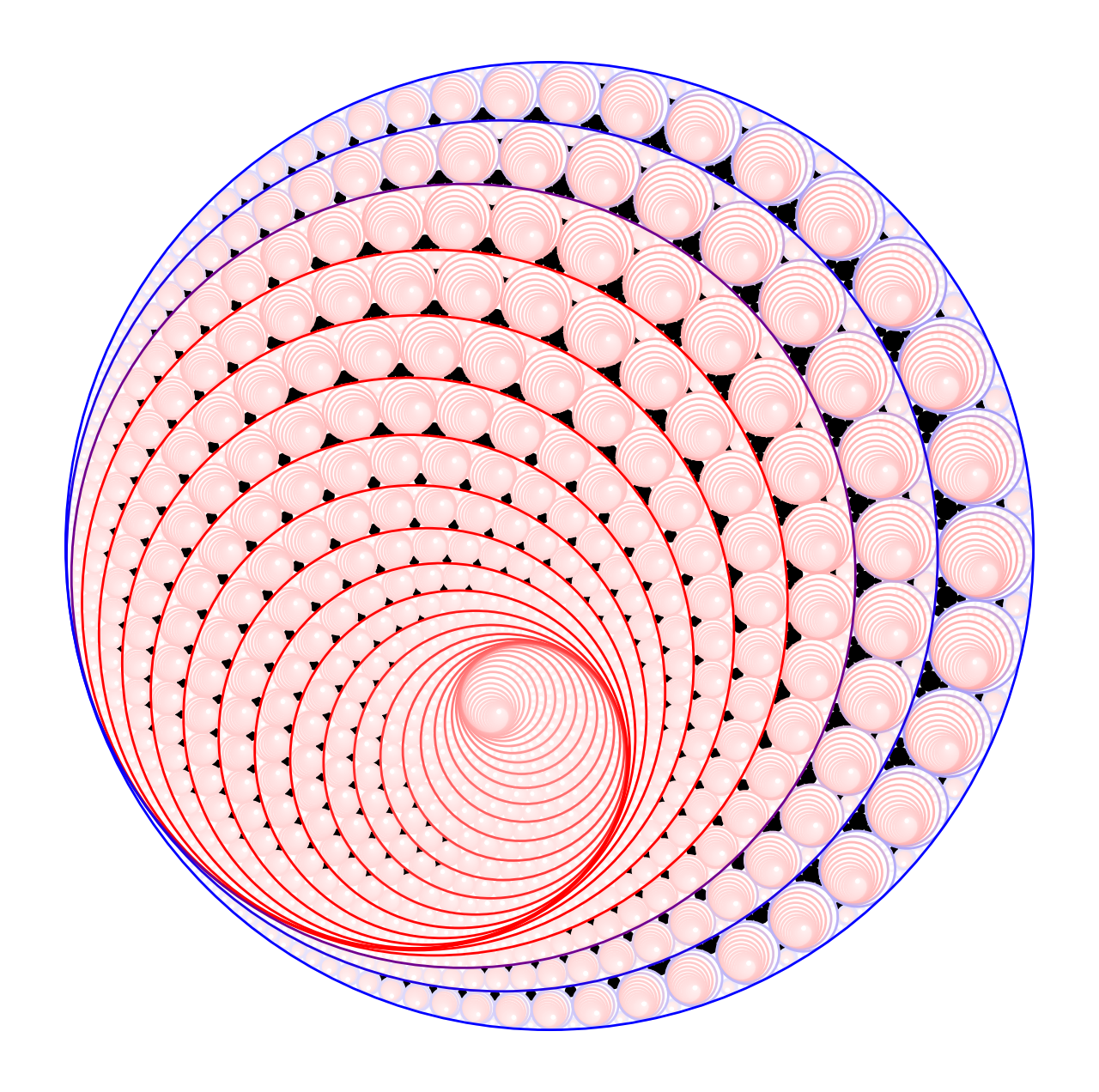
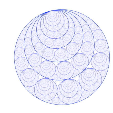
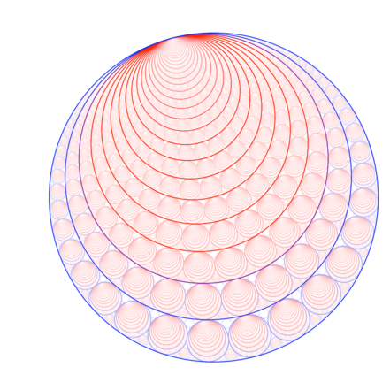
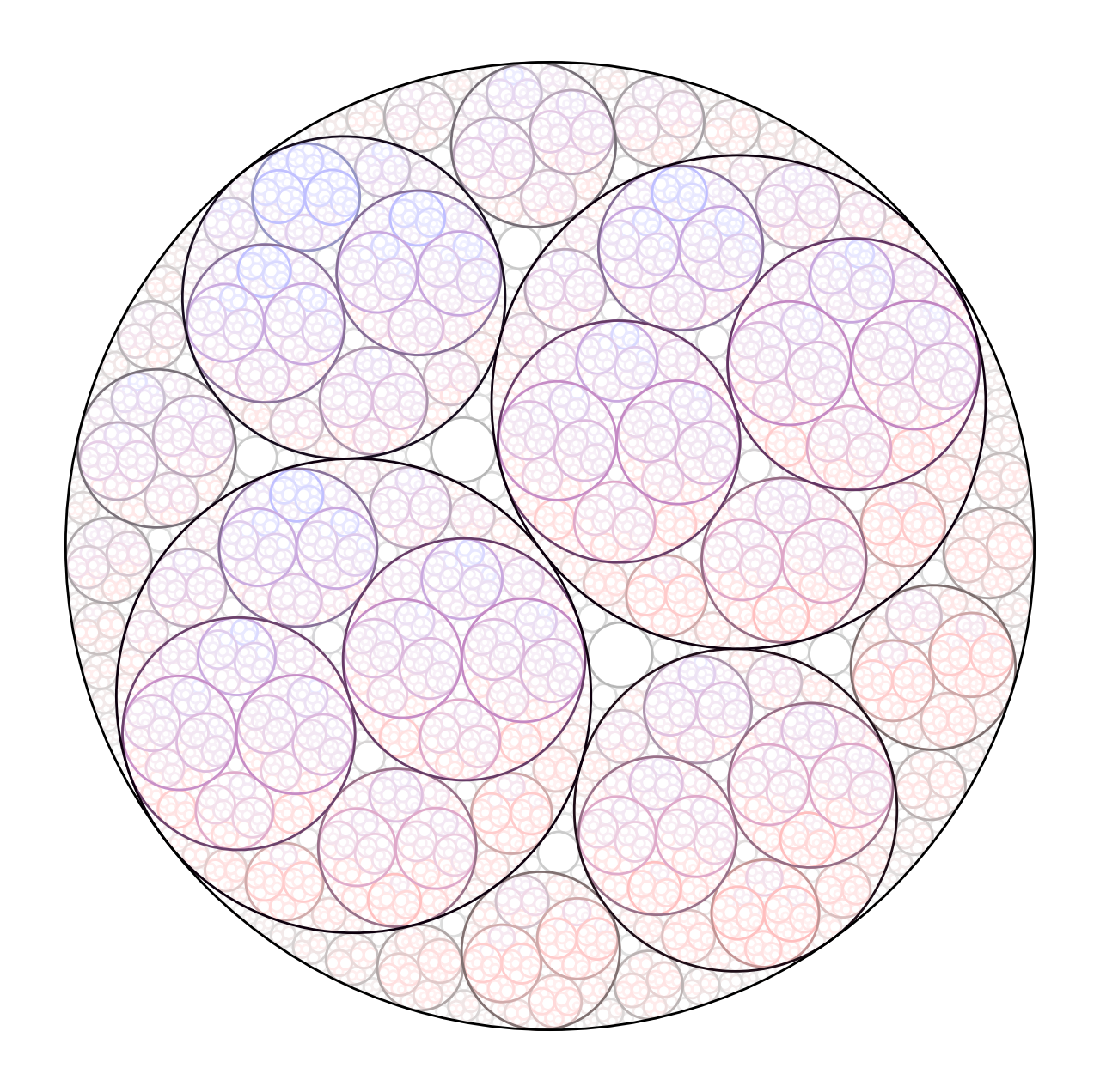
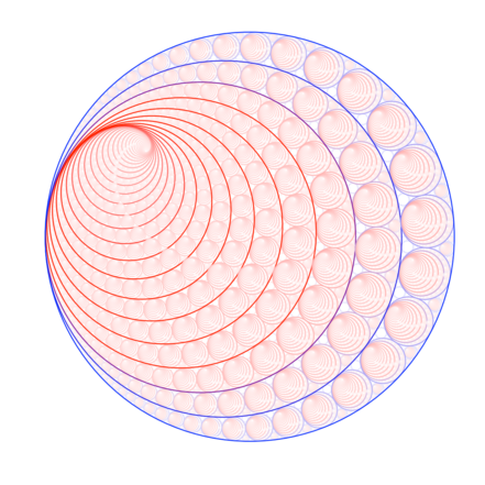
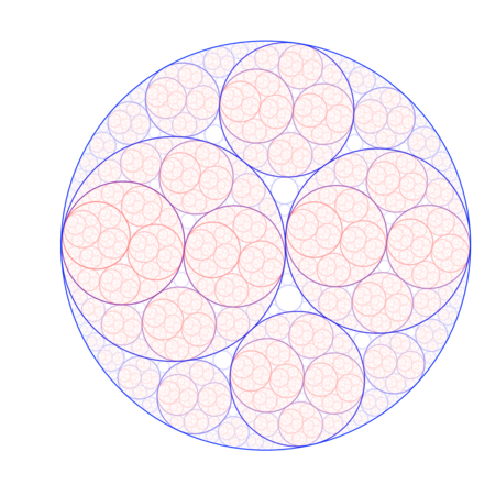
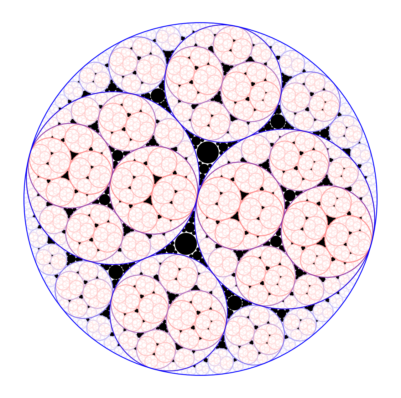
Animations of filled Apollonian gasket fractals Click on any image to play the corresponding .mp4 animation. Files are between 65 and 105 MB large. They are also be started by clicking the following links: 11, 12, 13, 14, 15, 17, 19, and 20.
Diffusion limited aggregation along a sticky wall	Modified aggregation to increase the fractal dimension
Tadpole orbit	Horseshoe orbit
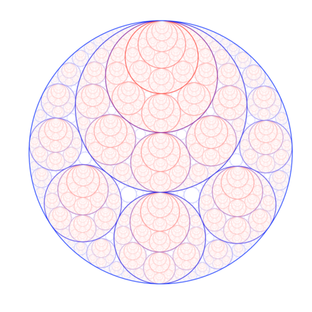
Molecular dynamics simulations using a Lennard-Jones pair potential	Apollonian gasket (here in higher resolution)
Protect yourself from lighting with a Faraday's cage by solving the Laplace equation ;=)	Dynamical simulation of the Lorenz equation
Diffusion limited aggregation along a sticky wall	Modified aggregation to increase the fractal dimension
Modified diffusion limited aggregation to grow more compact structures. Click on the images to start an animation.
Diffusion limited aggregation with two species. Click on each image to see the structures growing.
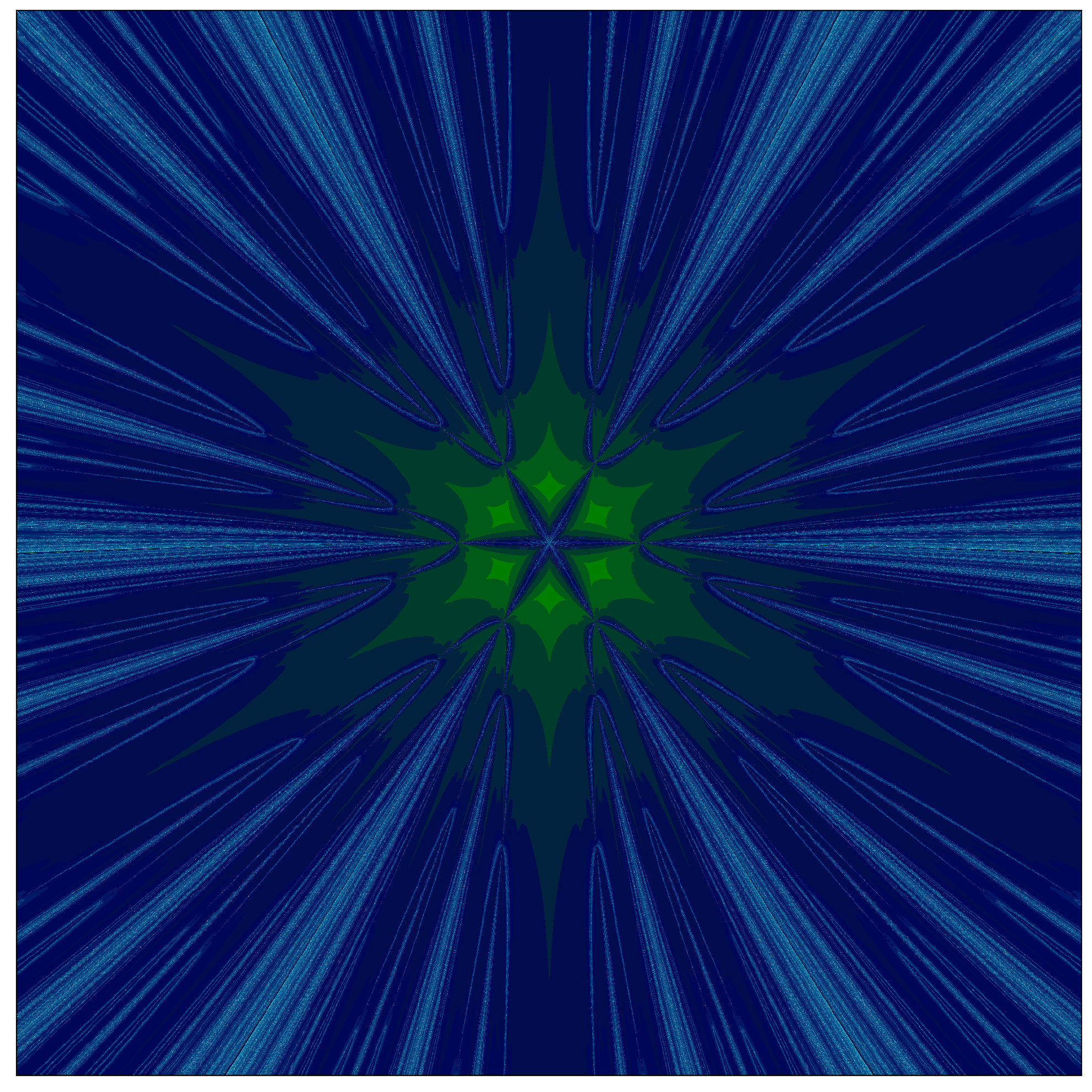
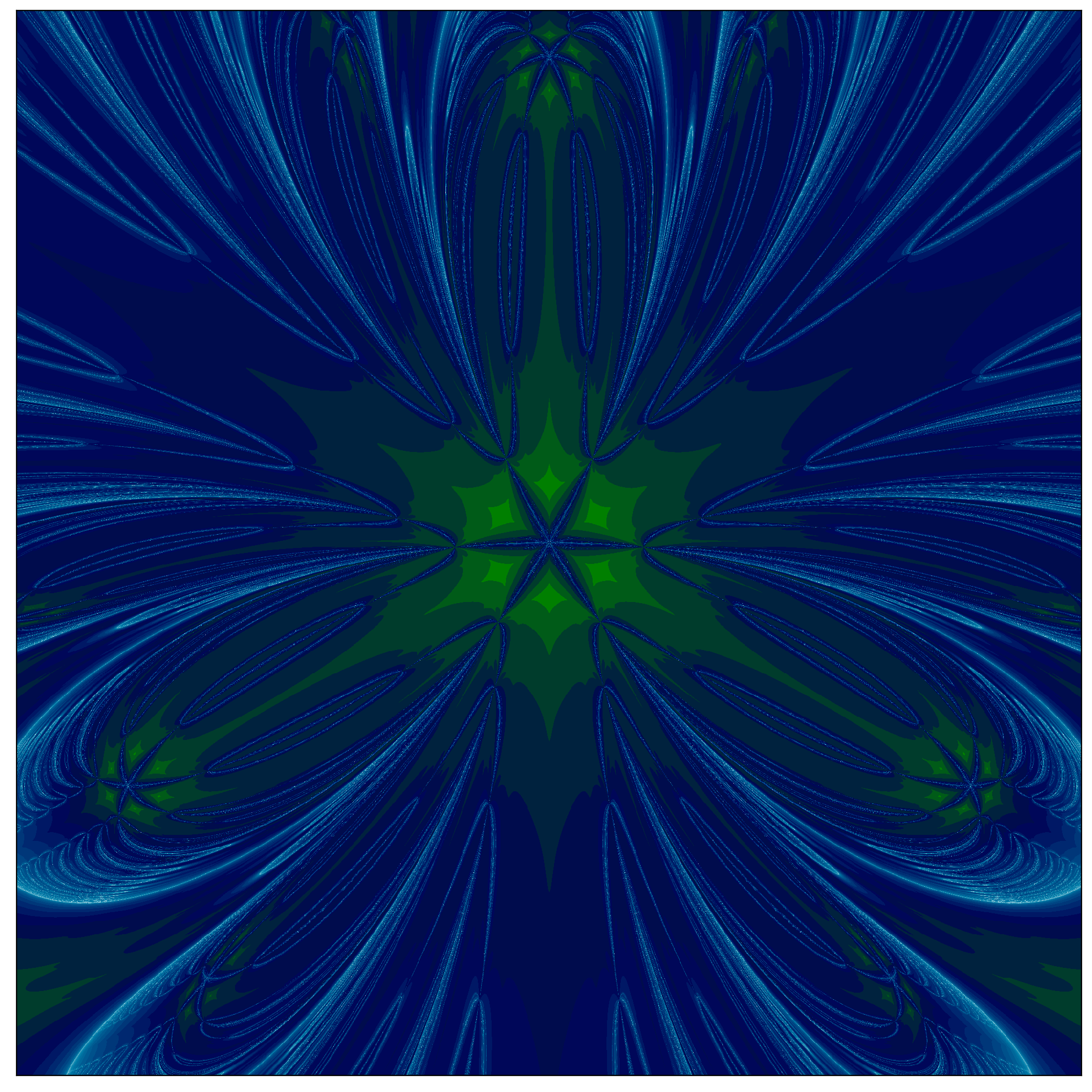
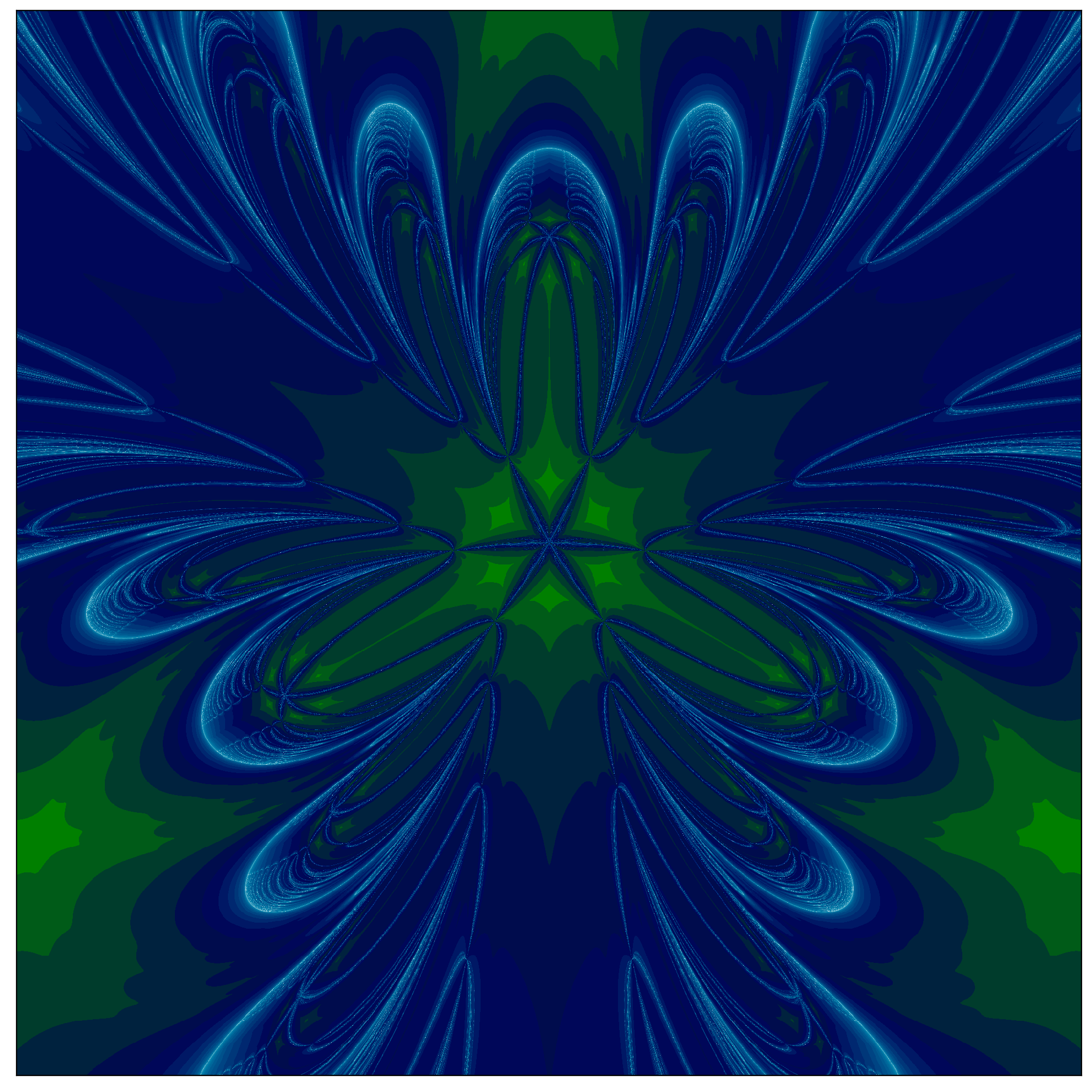
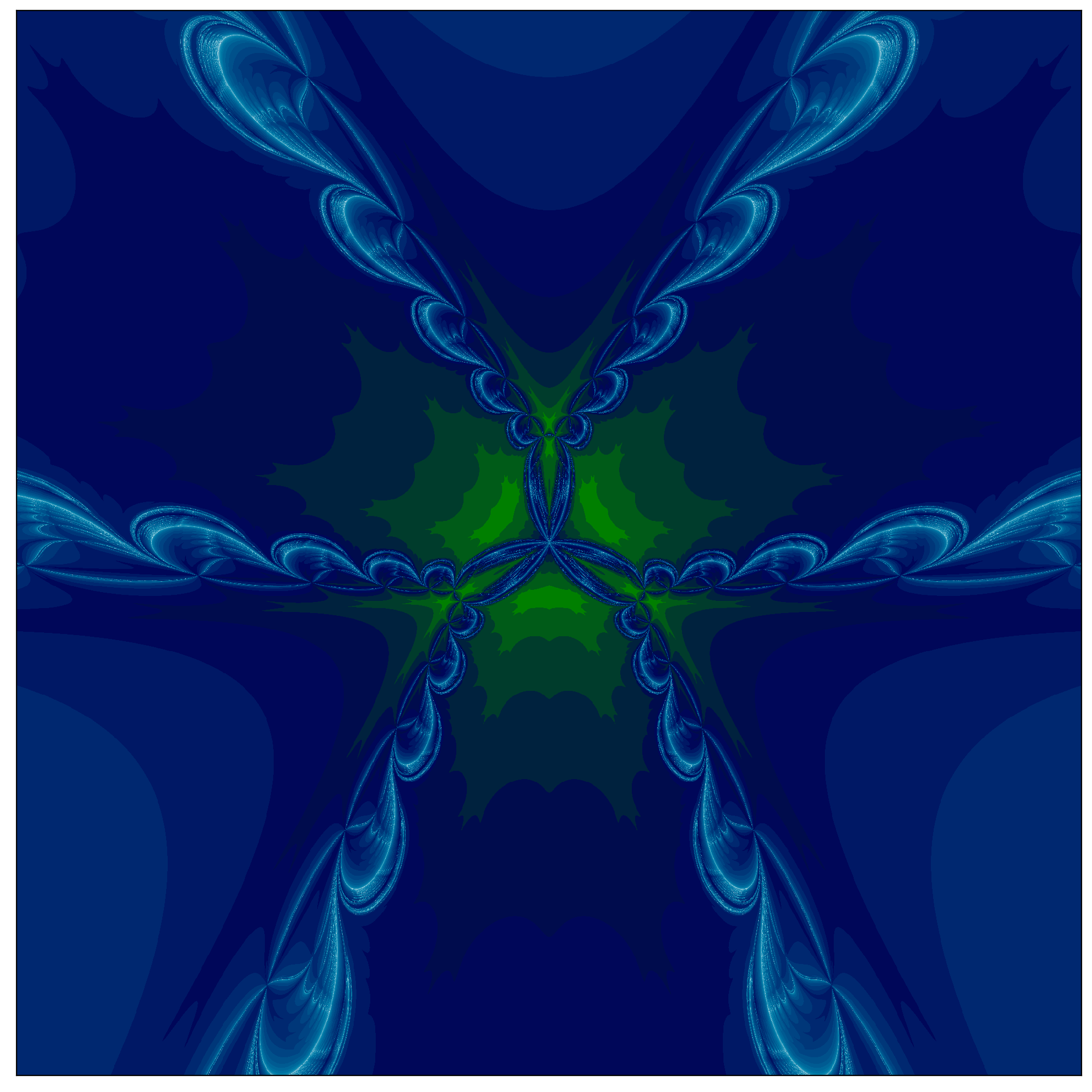
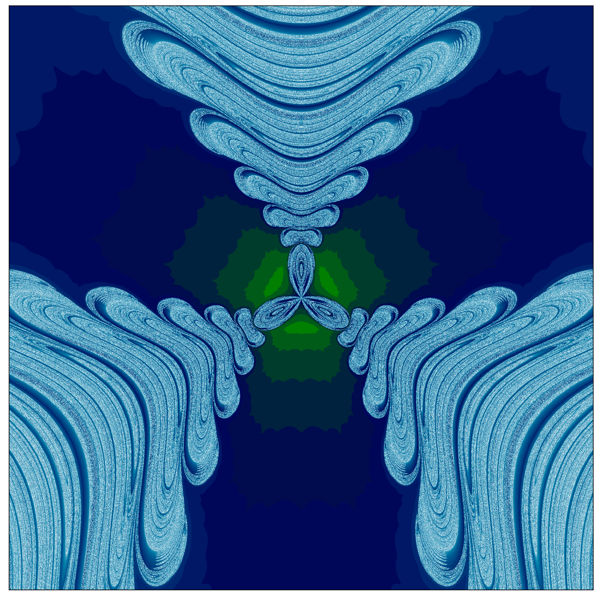
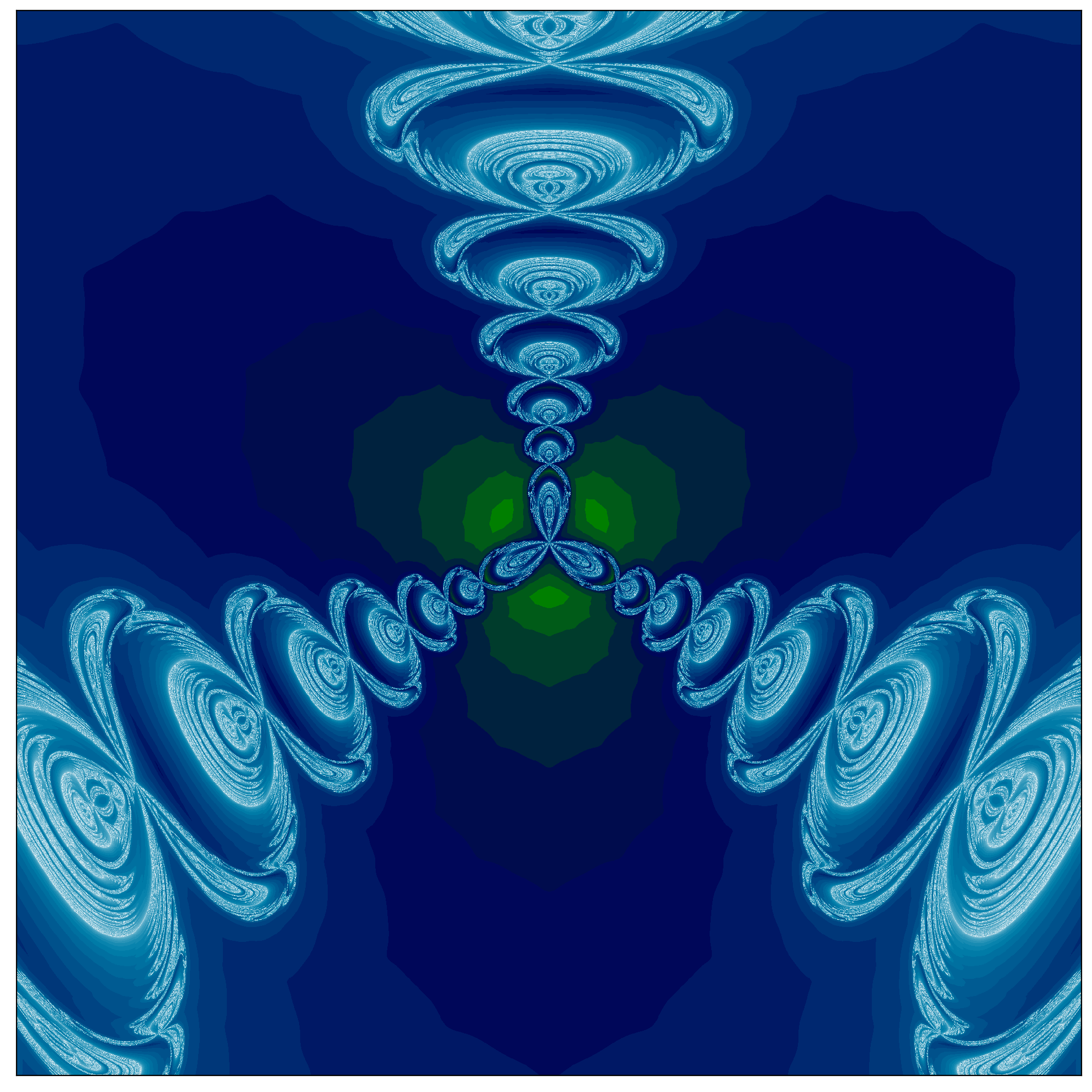
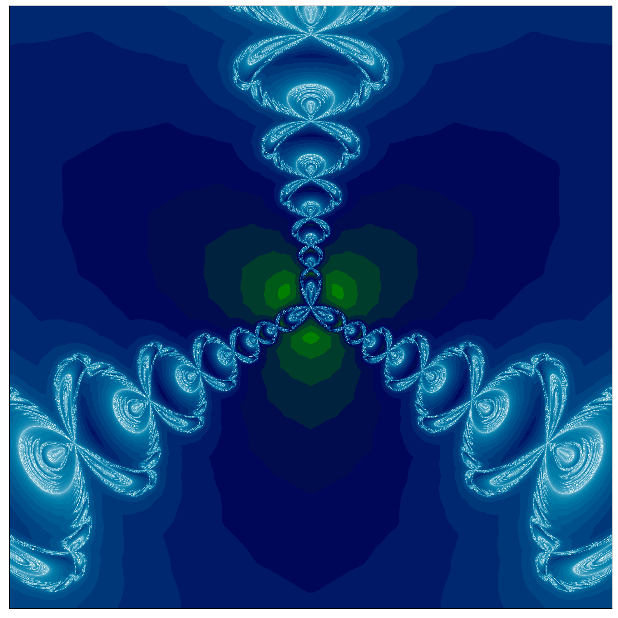
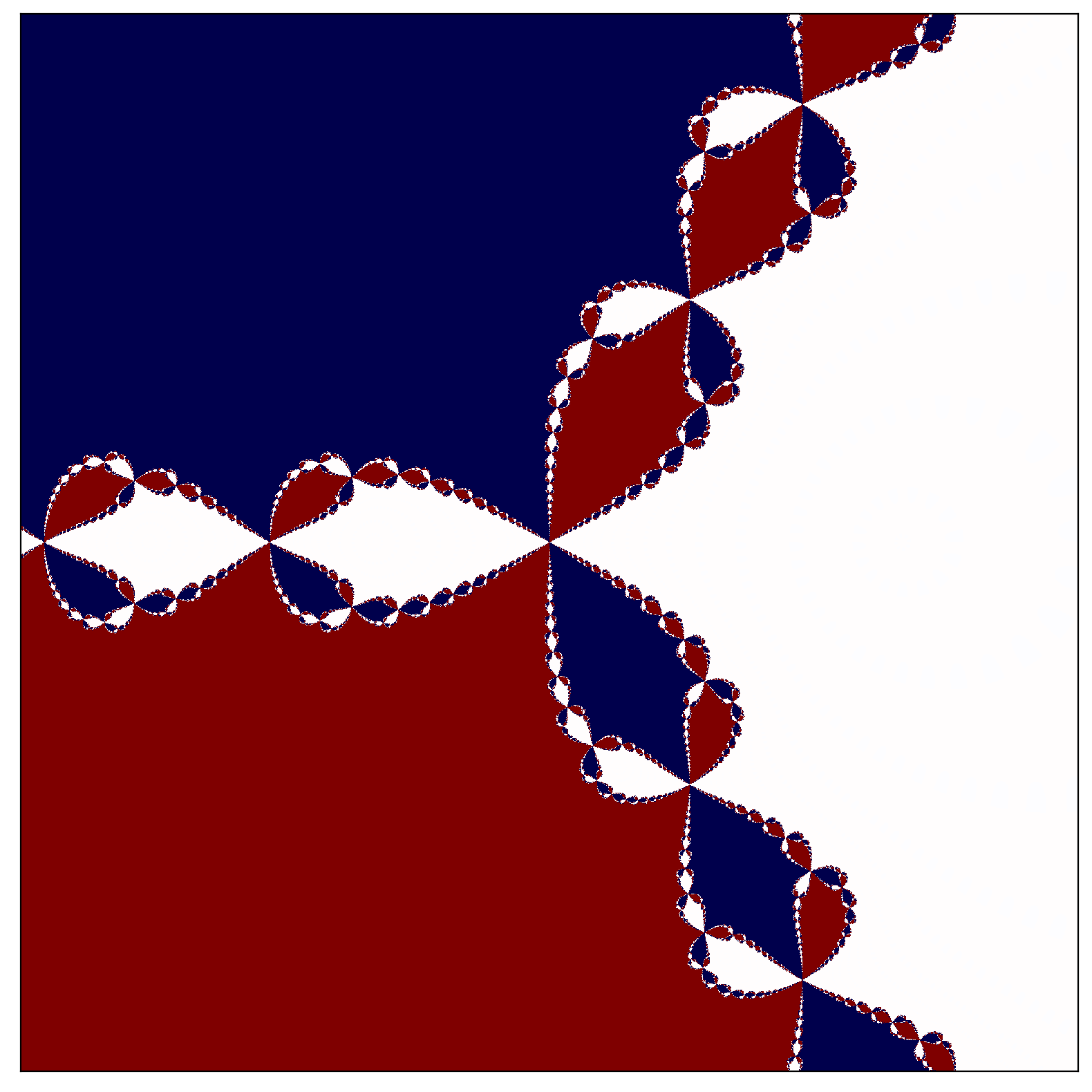
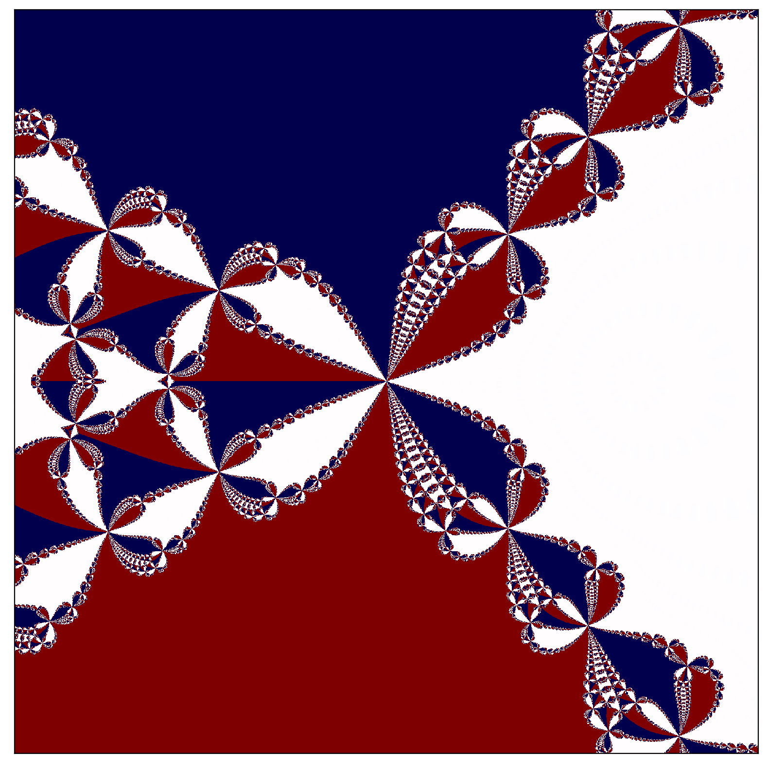
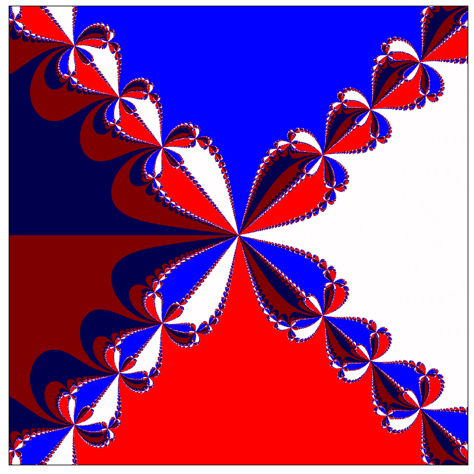
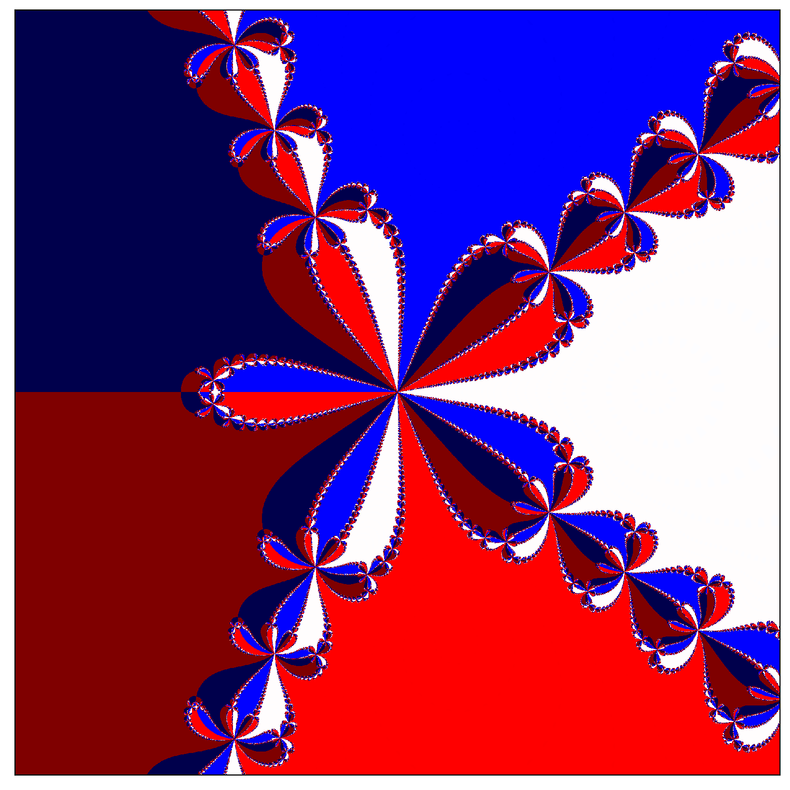
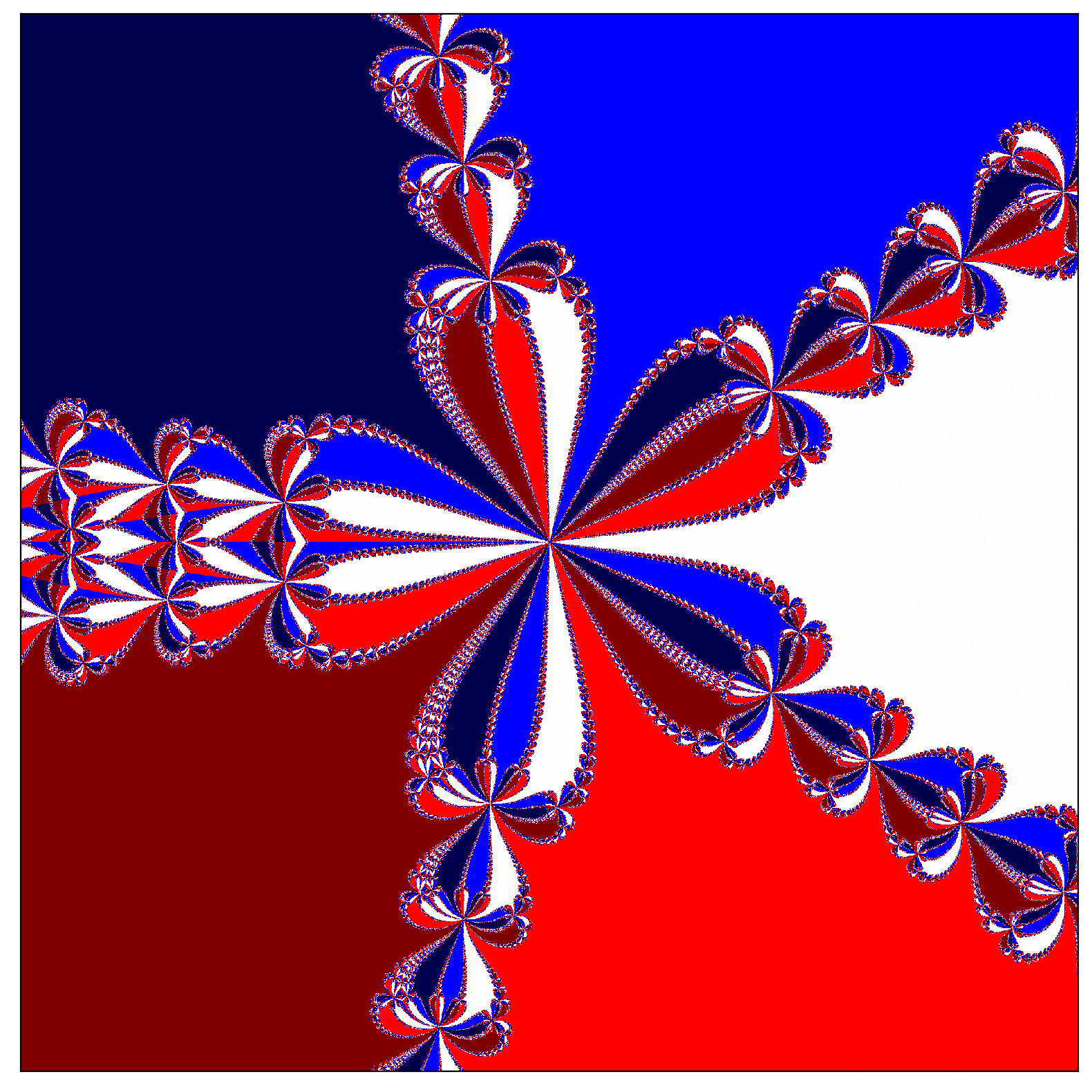
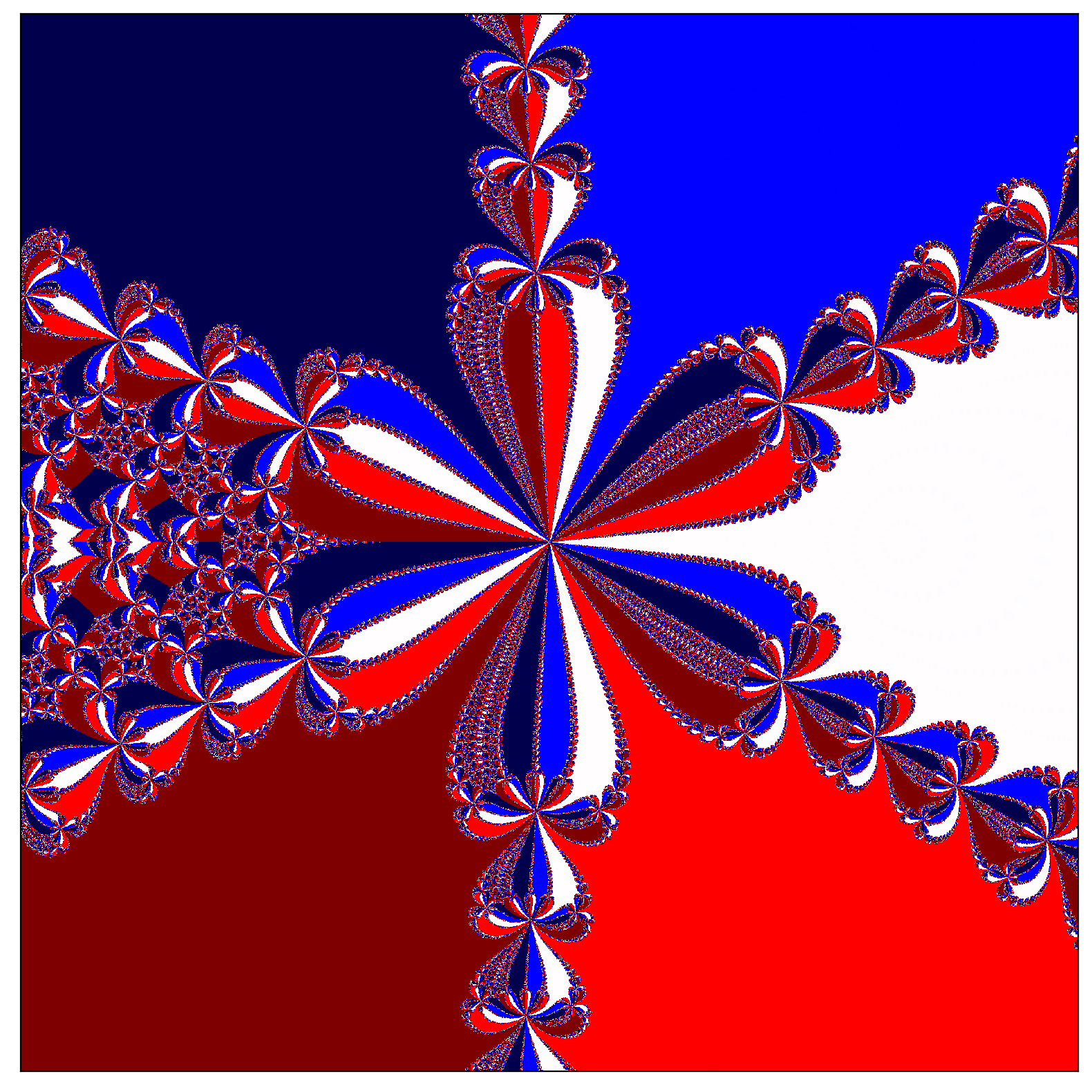
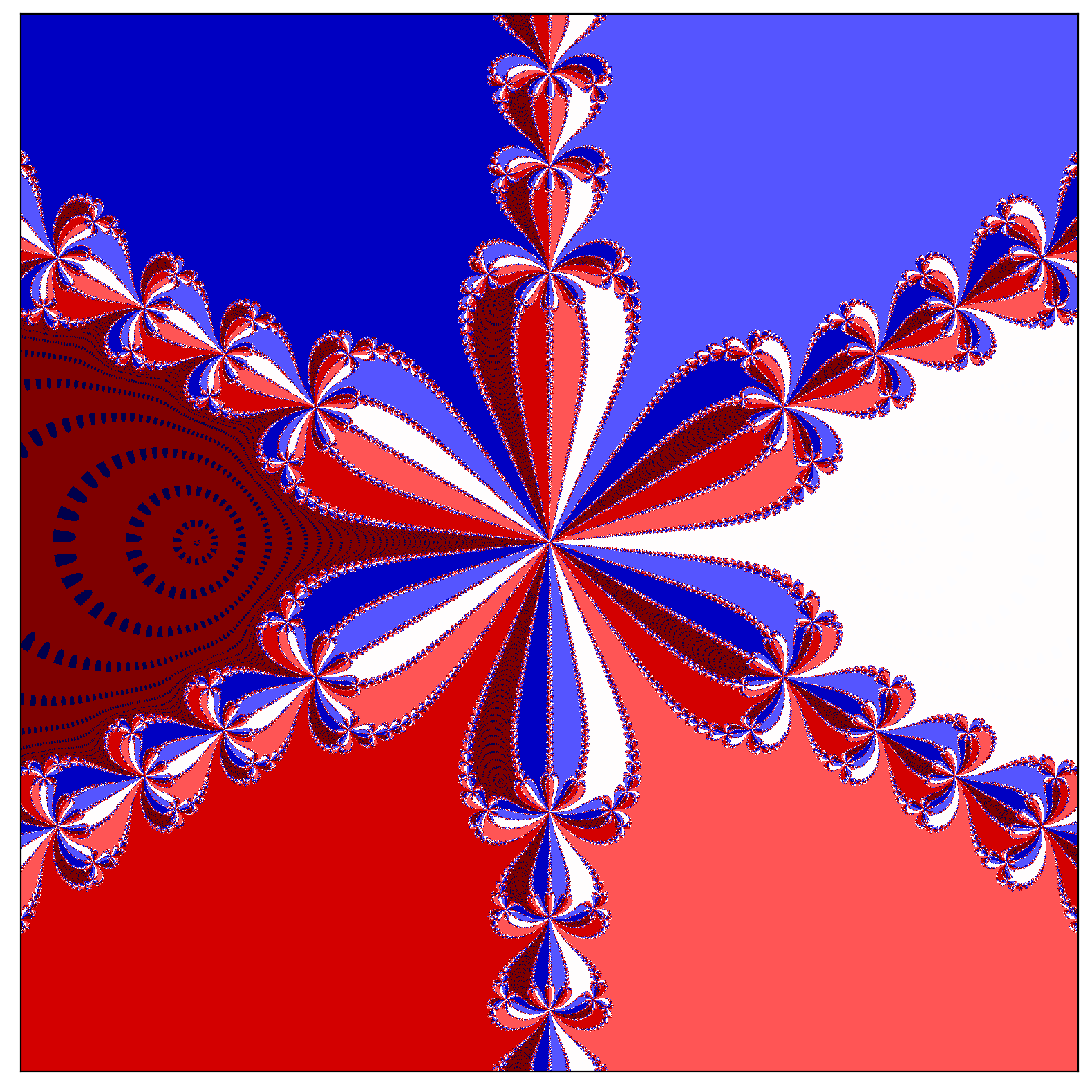
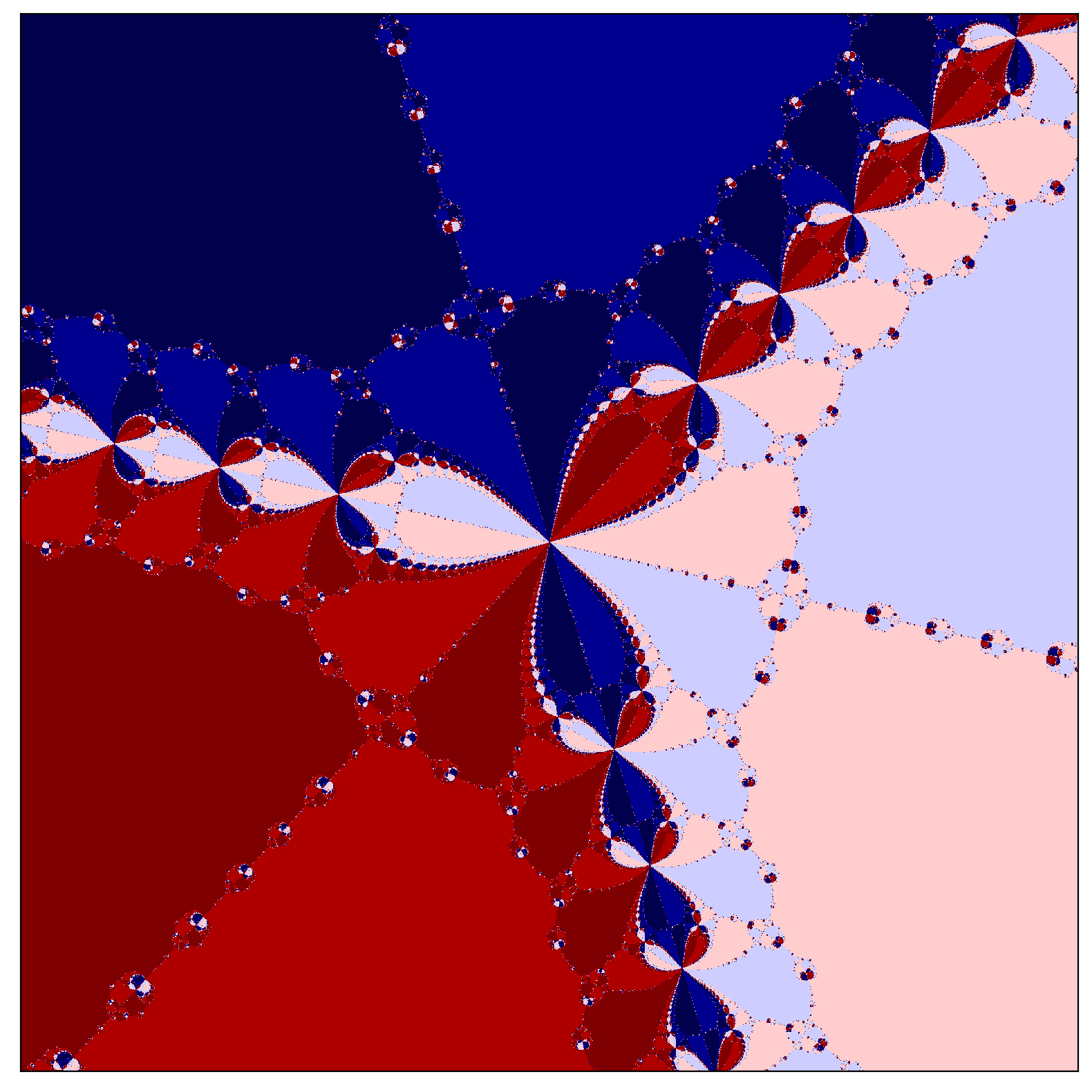
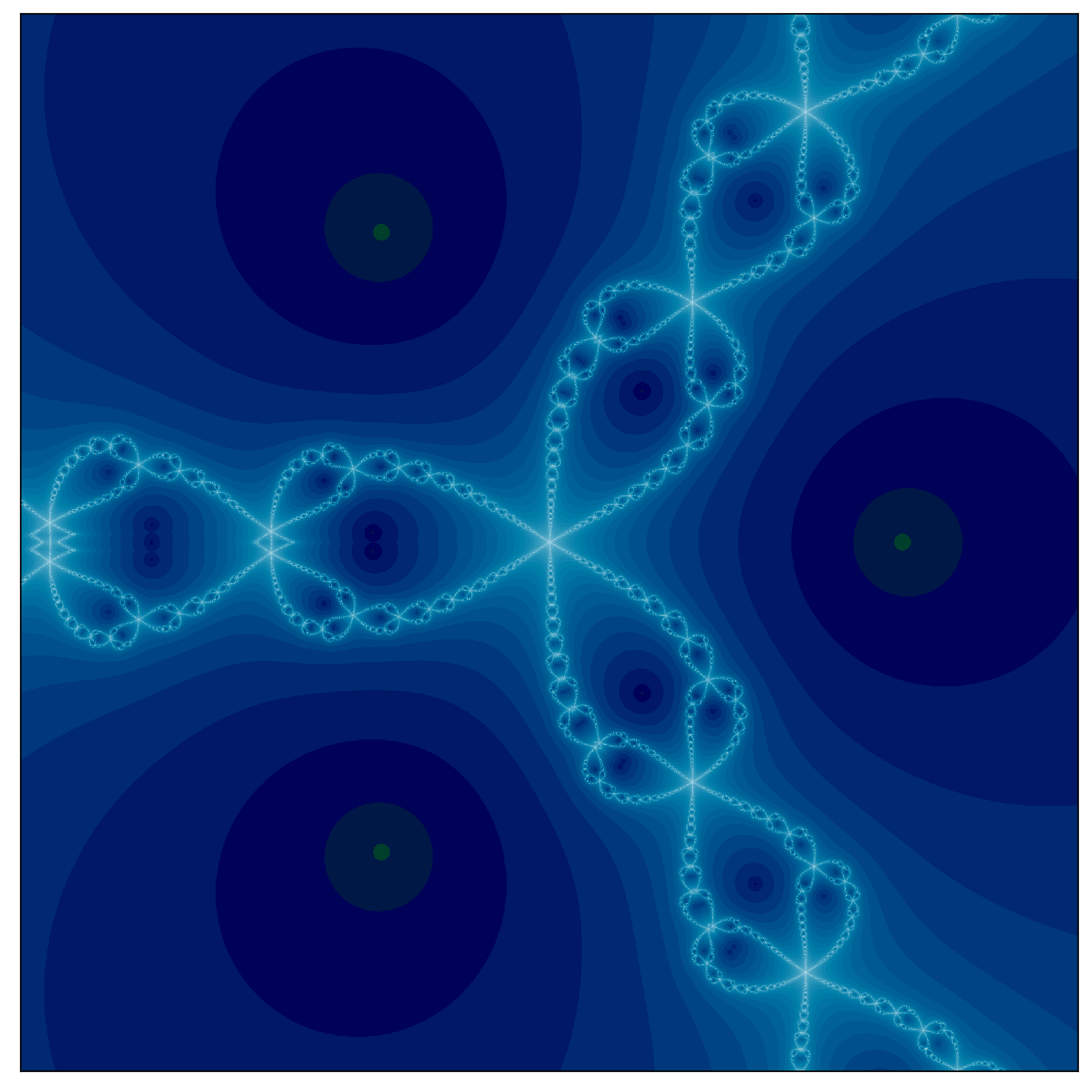
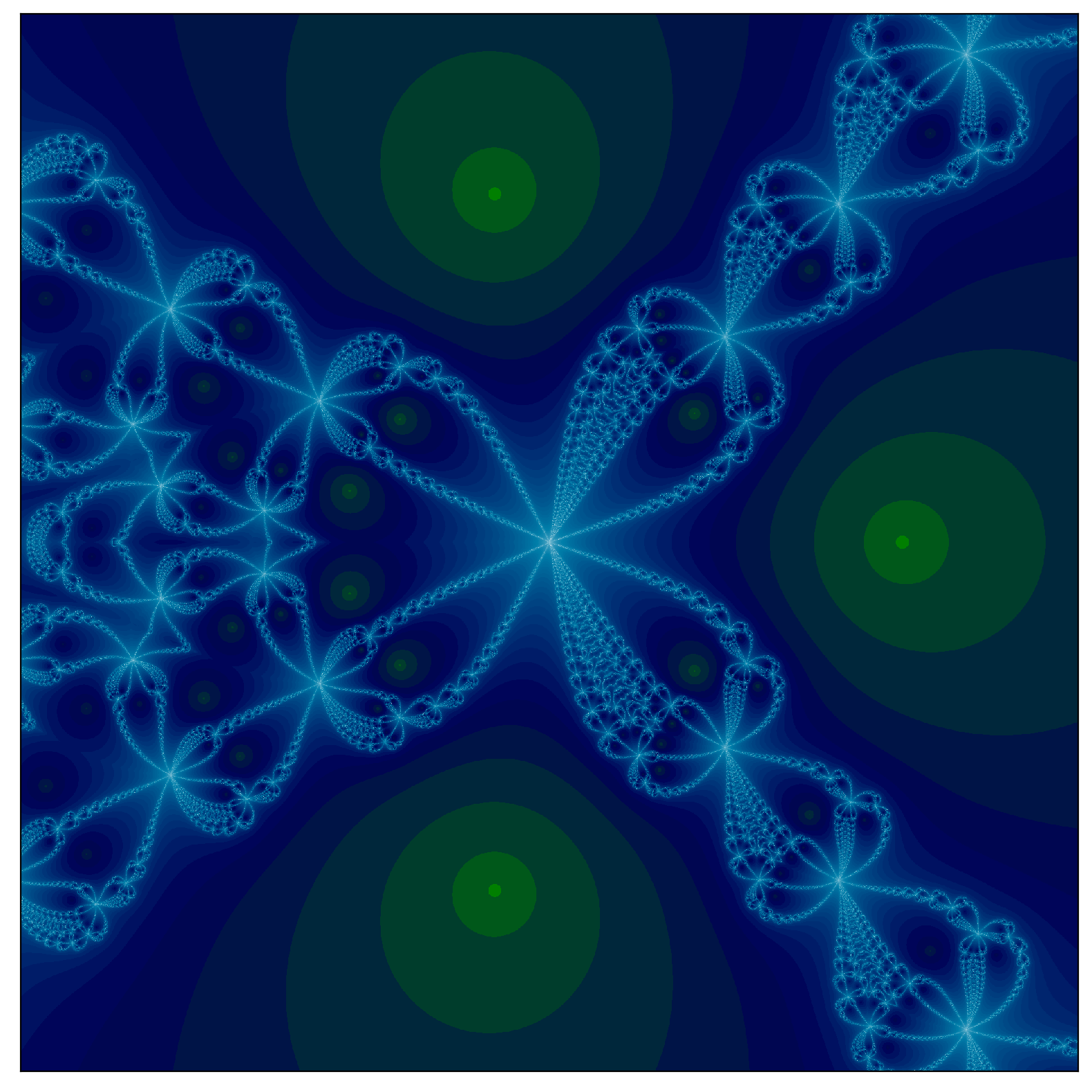
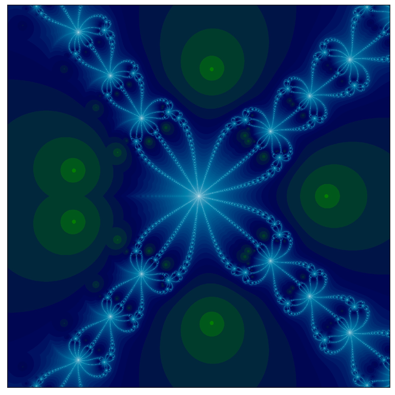
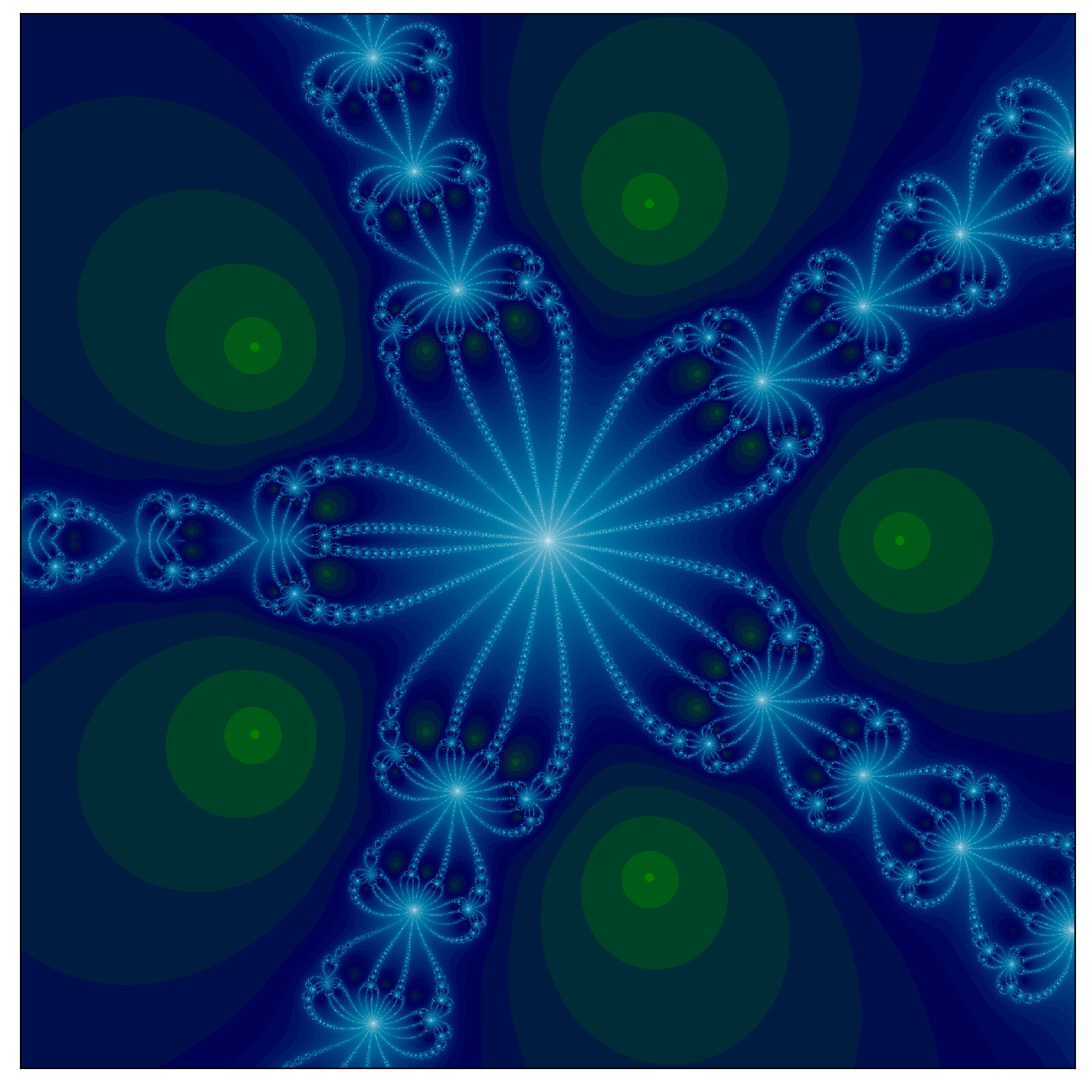
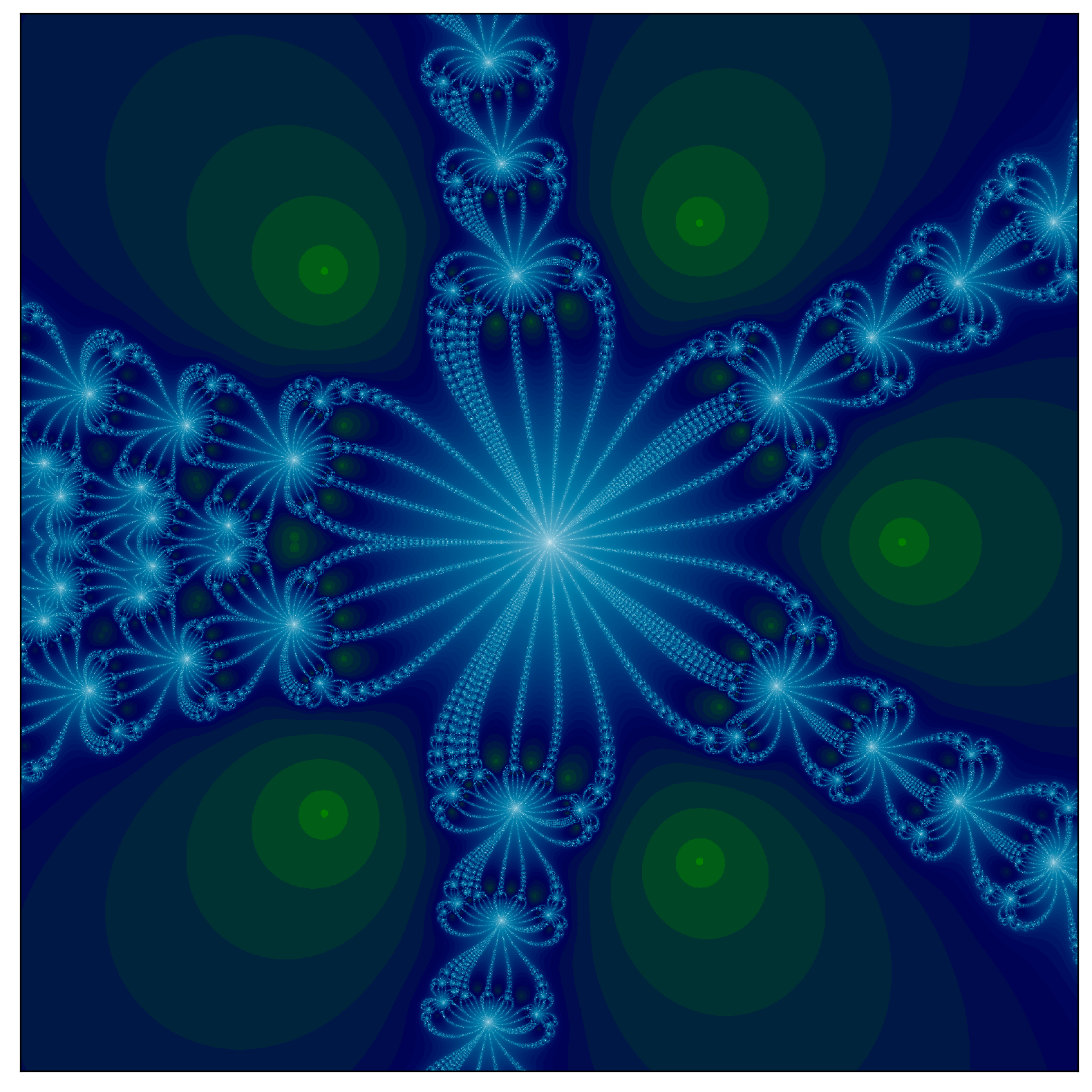
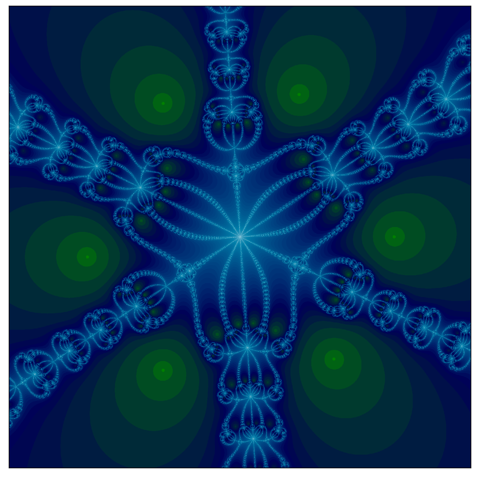
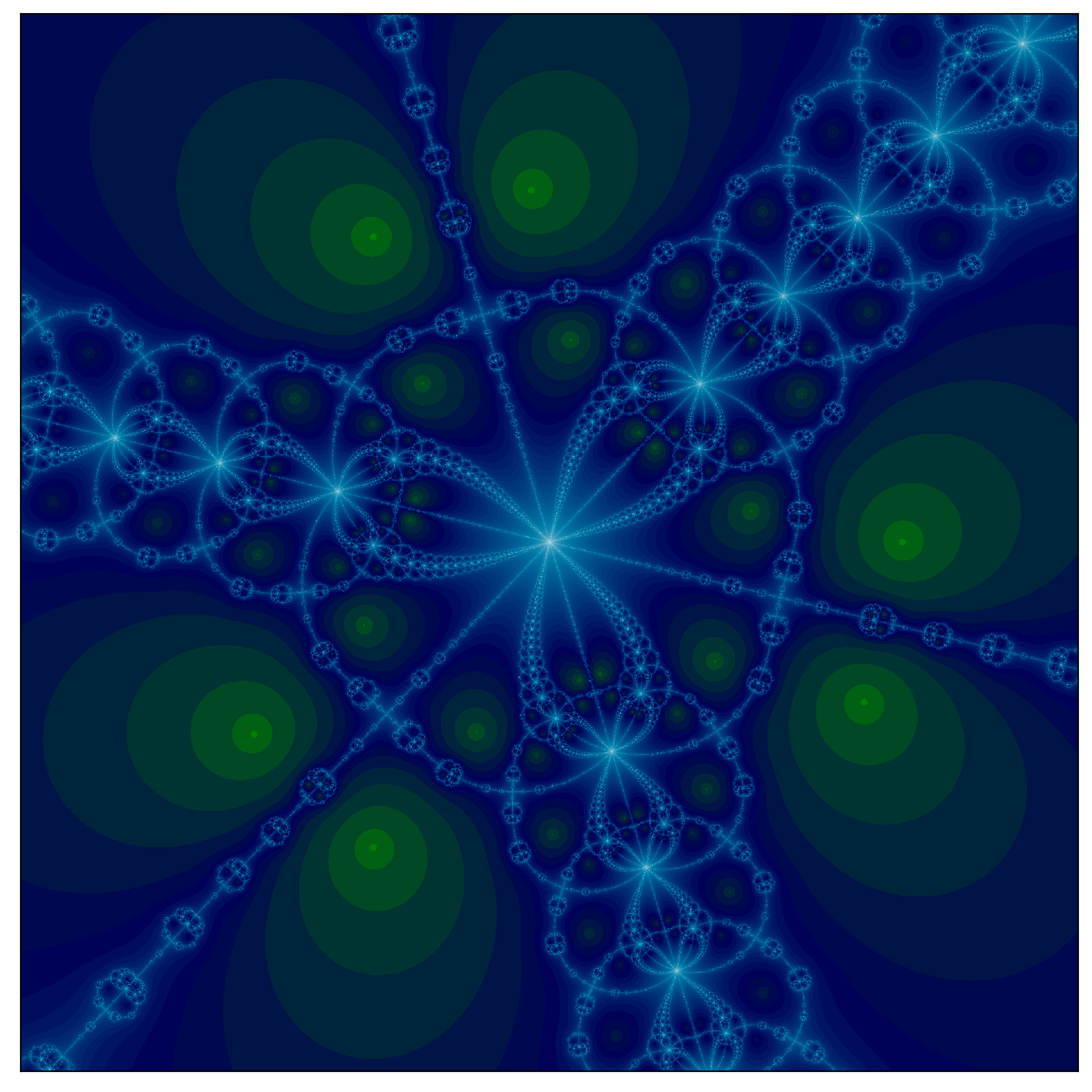
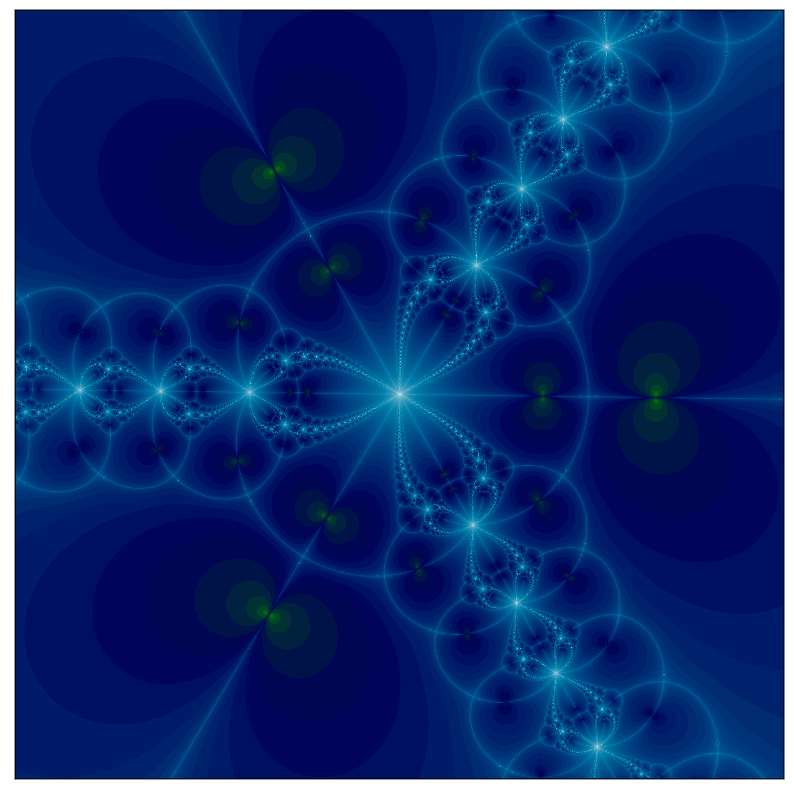
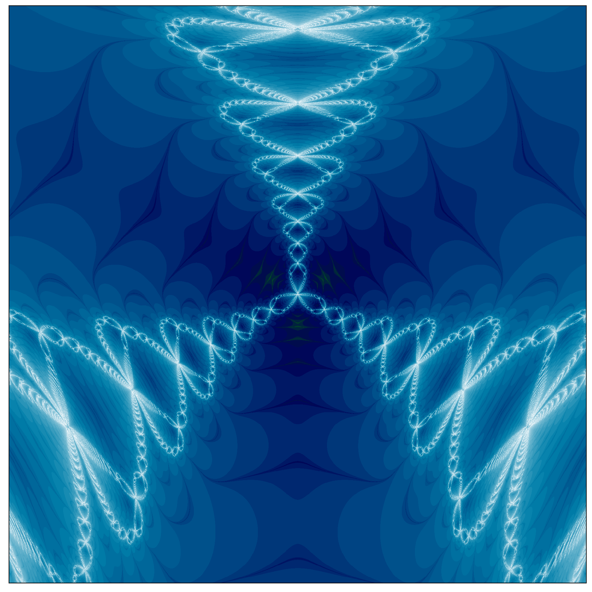
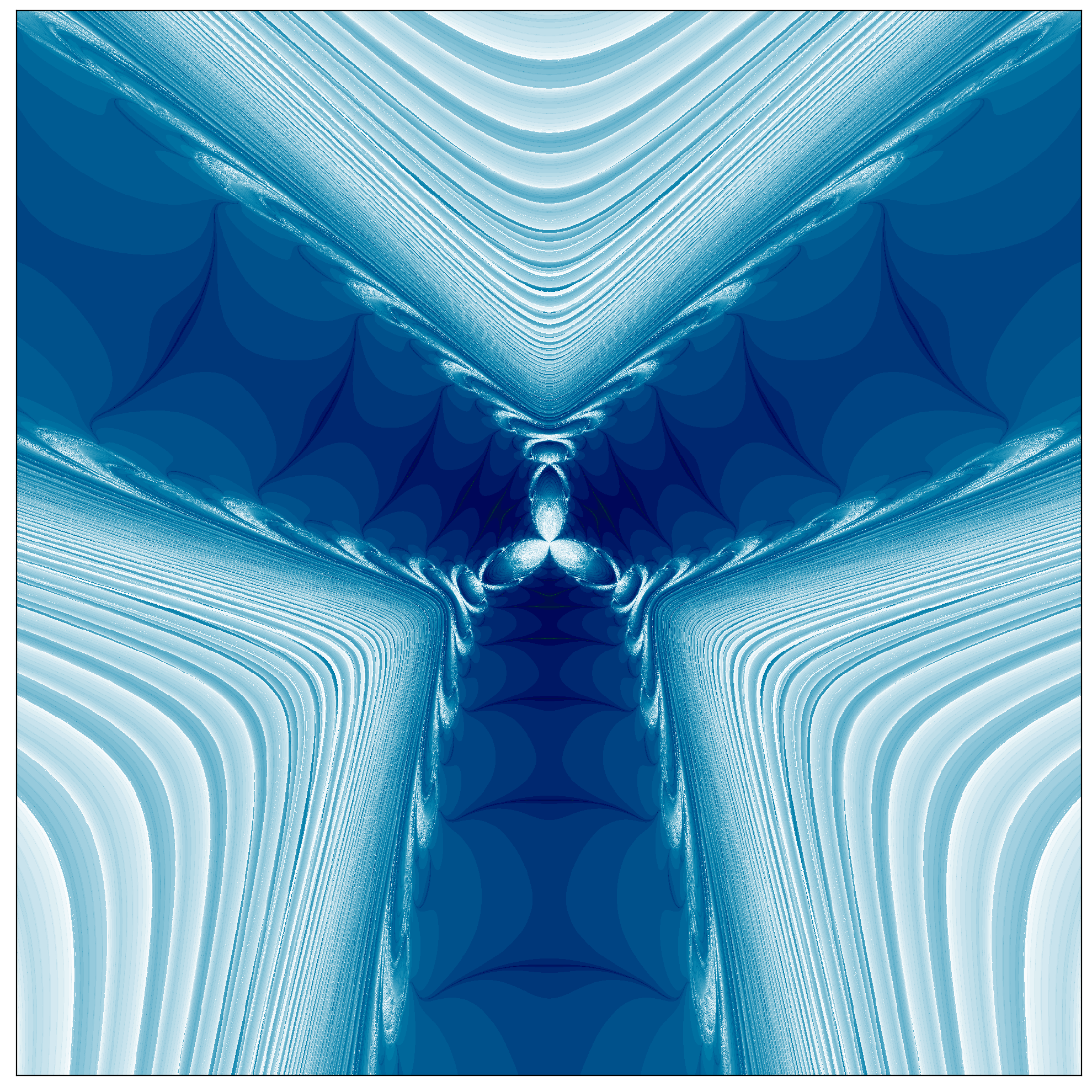
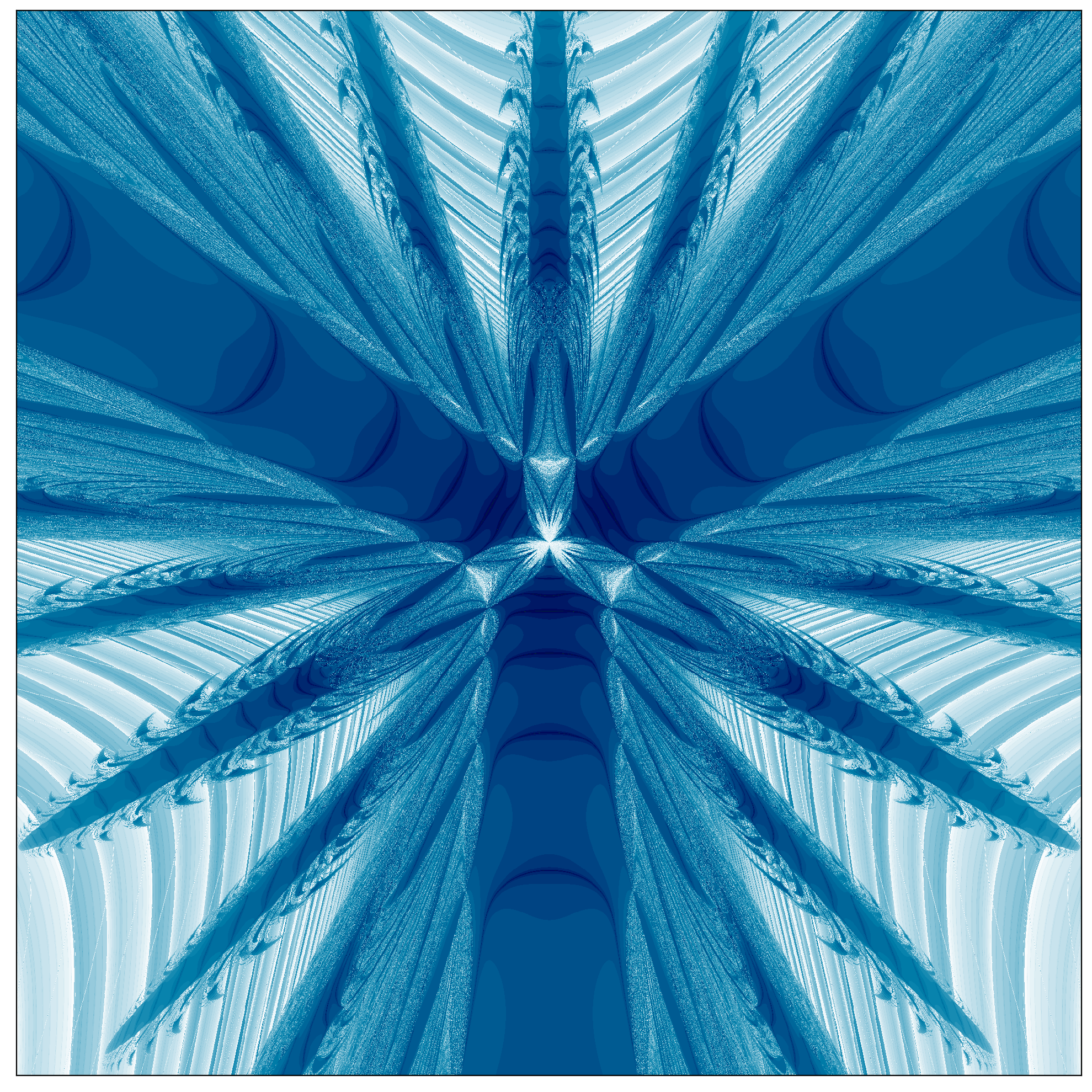
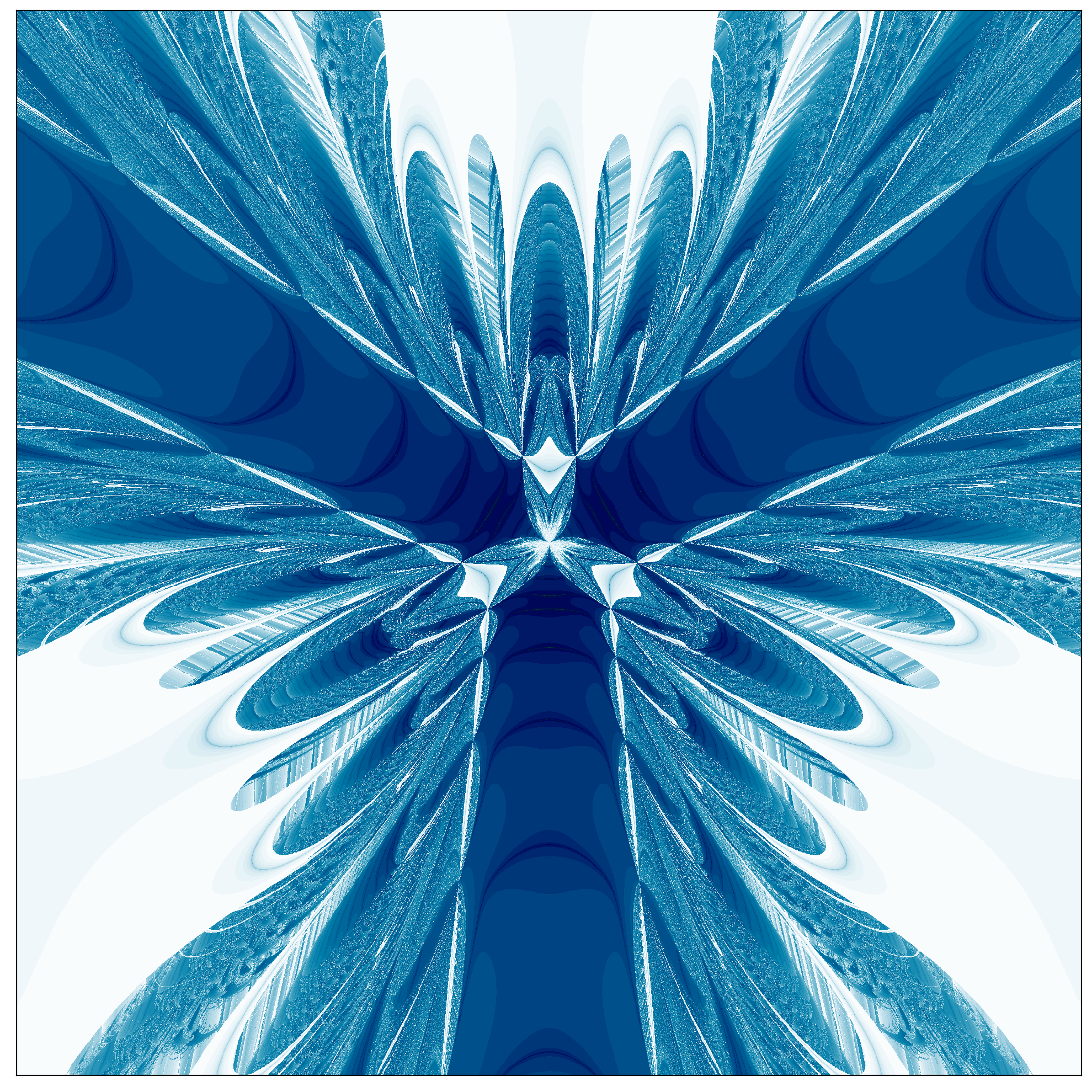
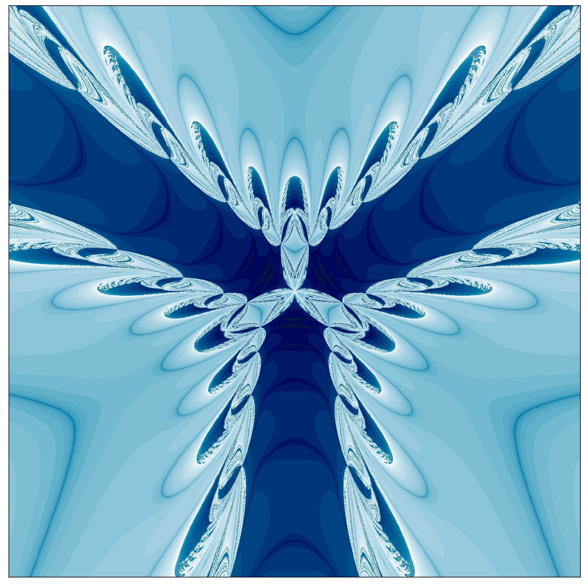
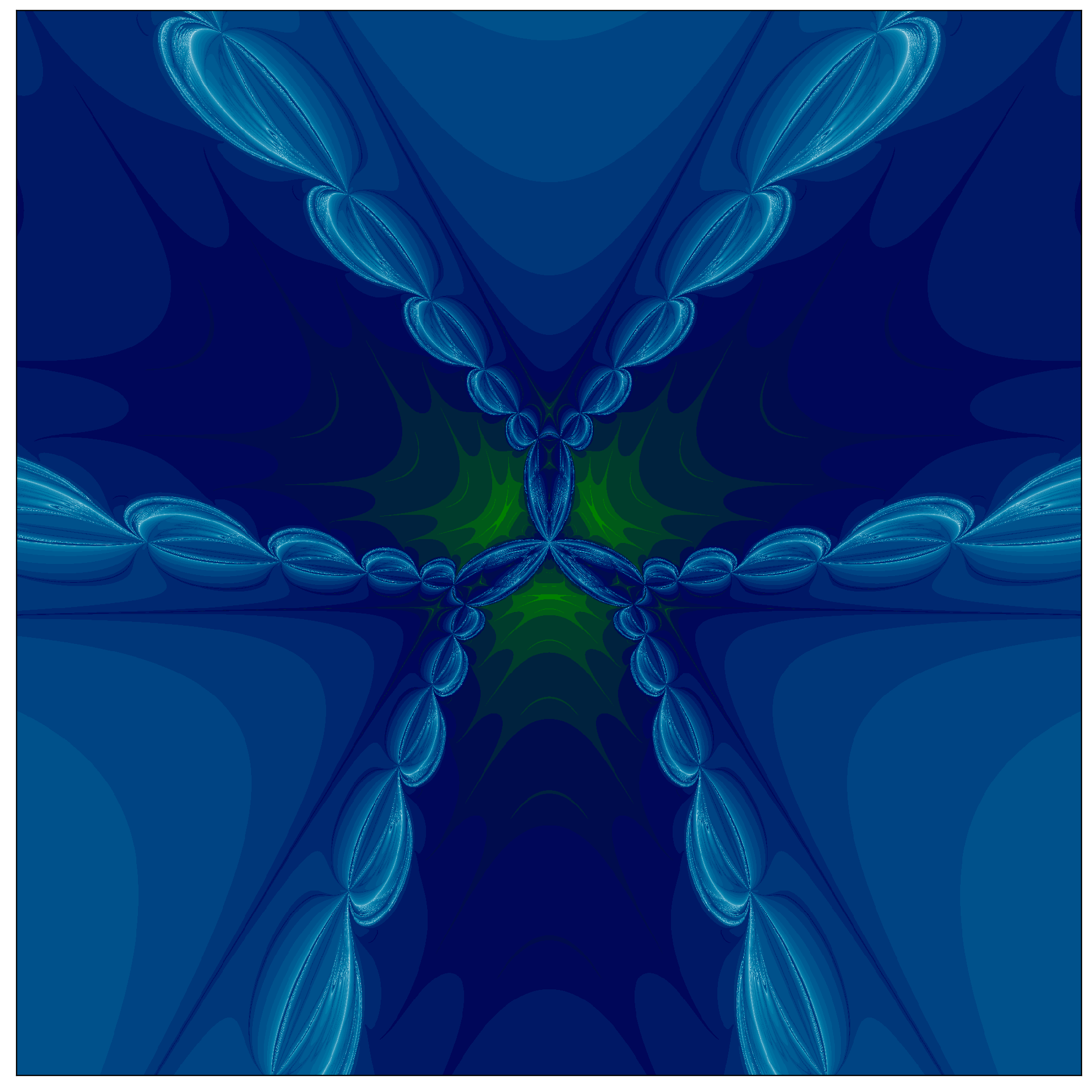
Series of fractals obtained with Newton's method in the complex plane. Click on any image in the upper two rows to see it in 2K resolution. Here are five animations: One, two, three, four, and five.
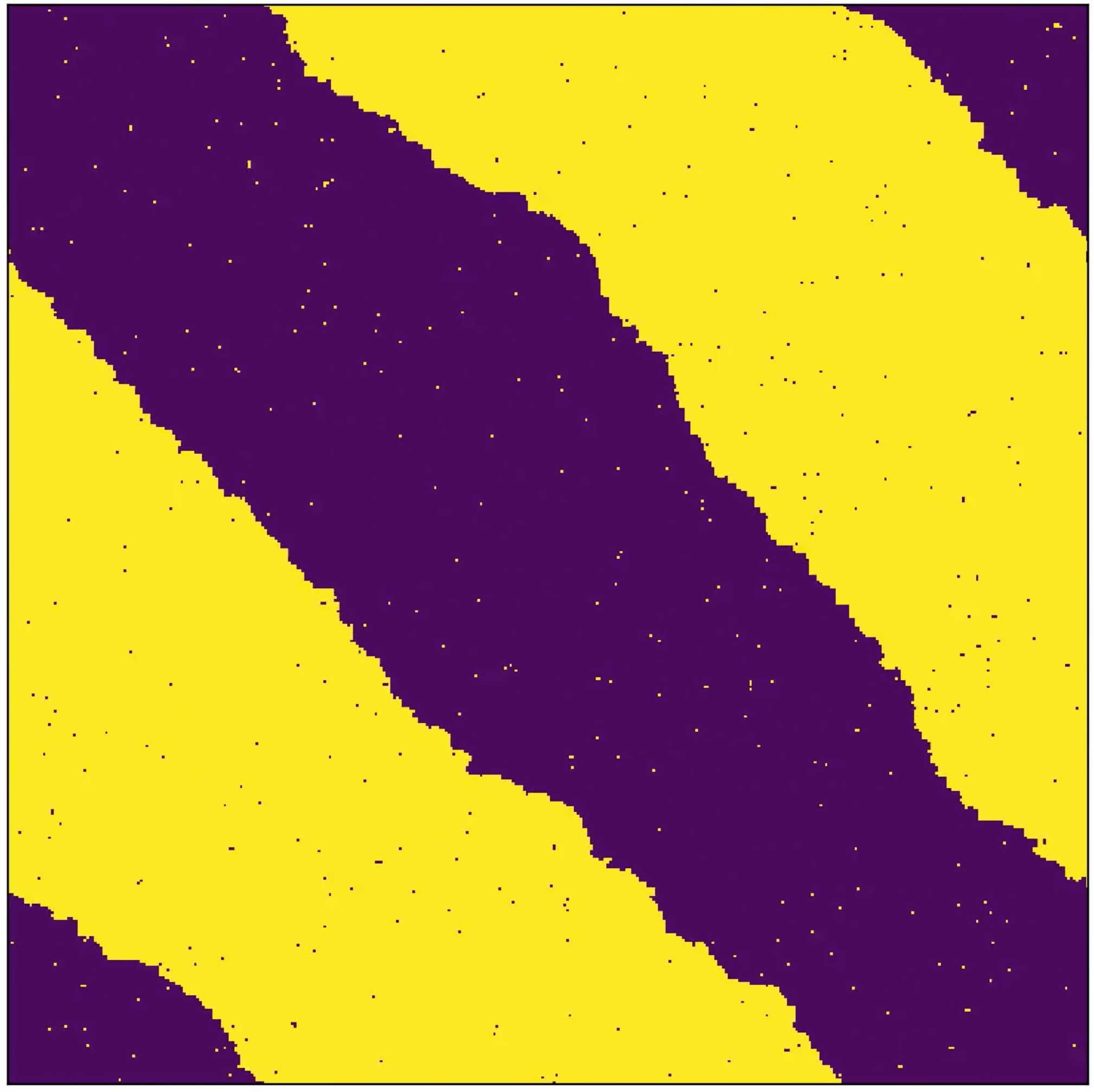
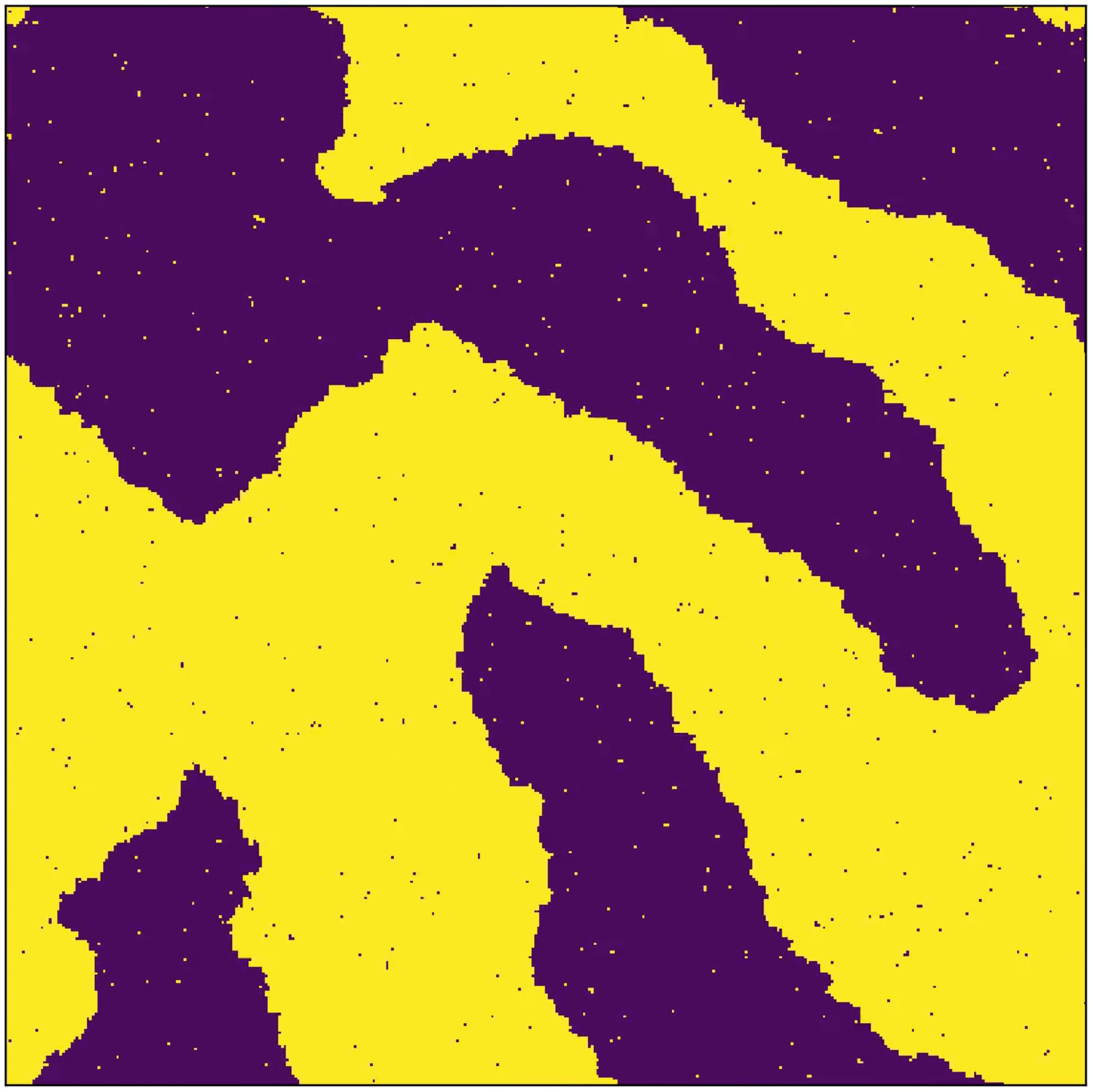
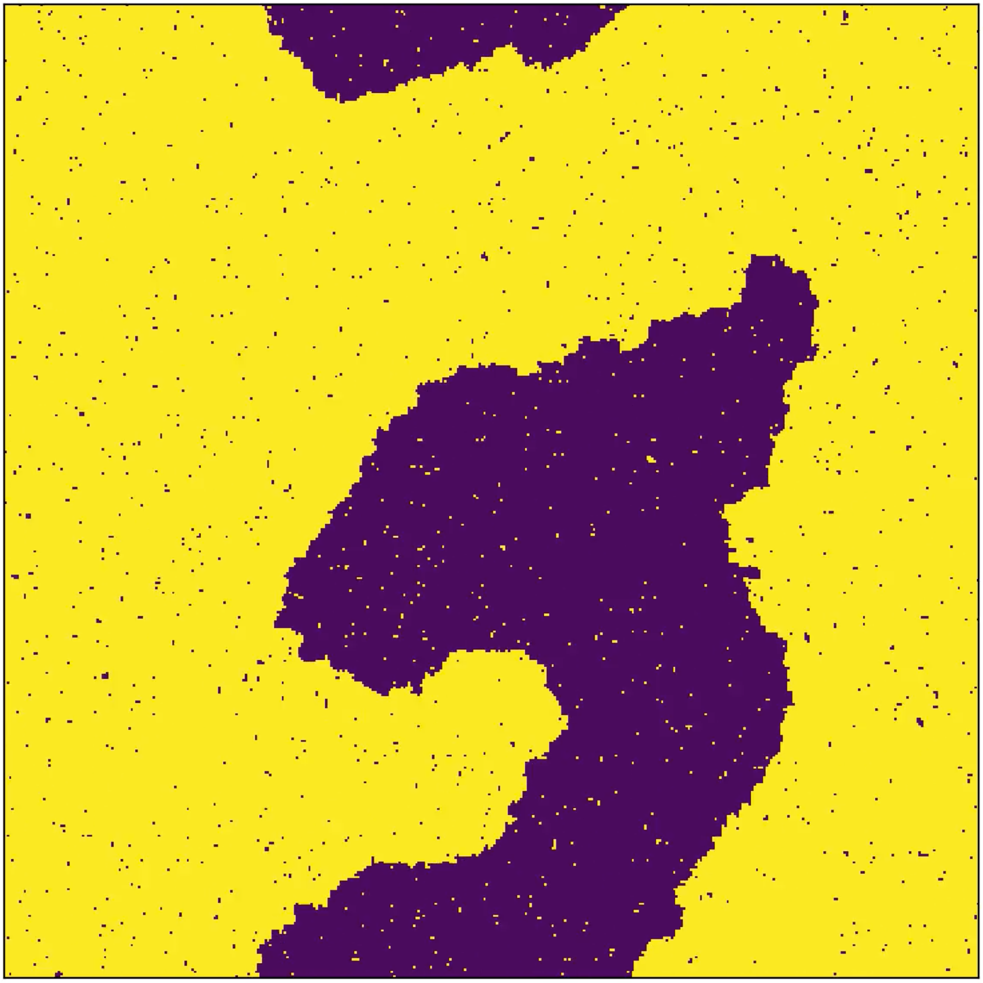
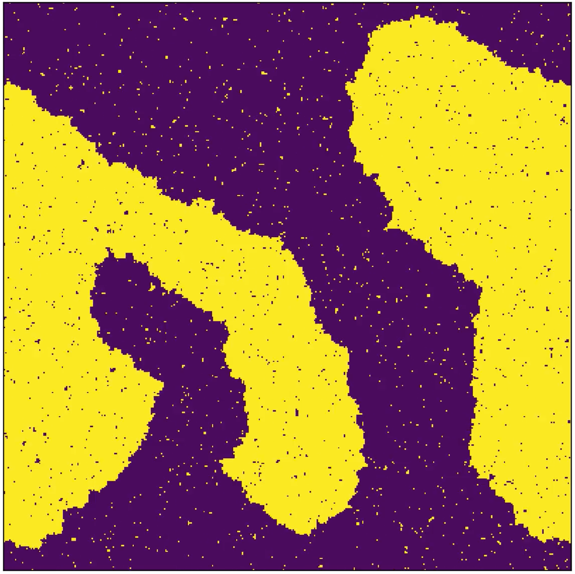
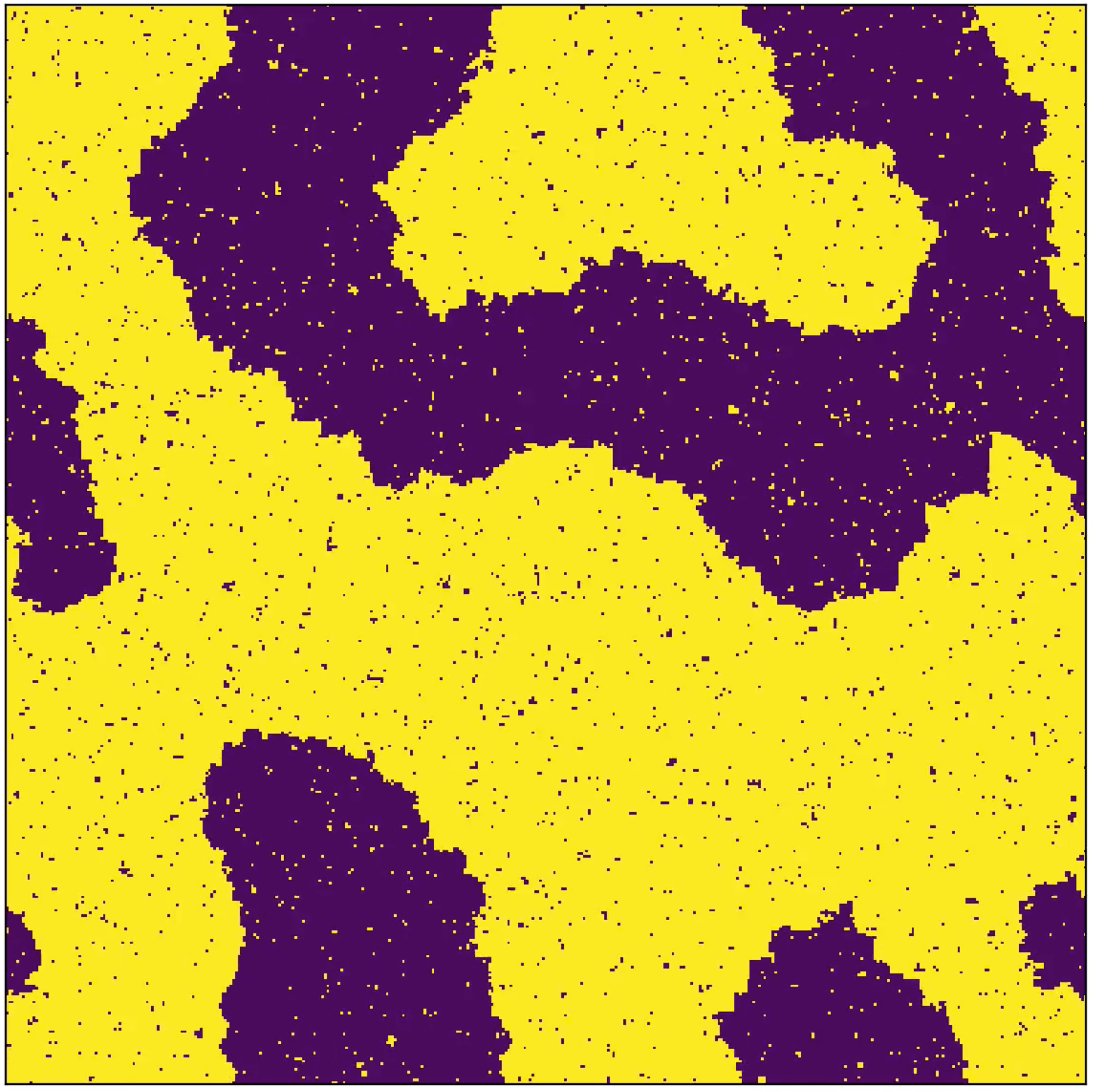
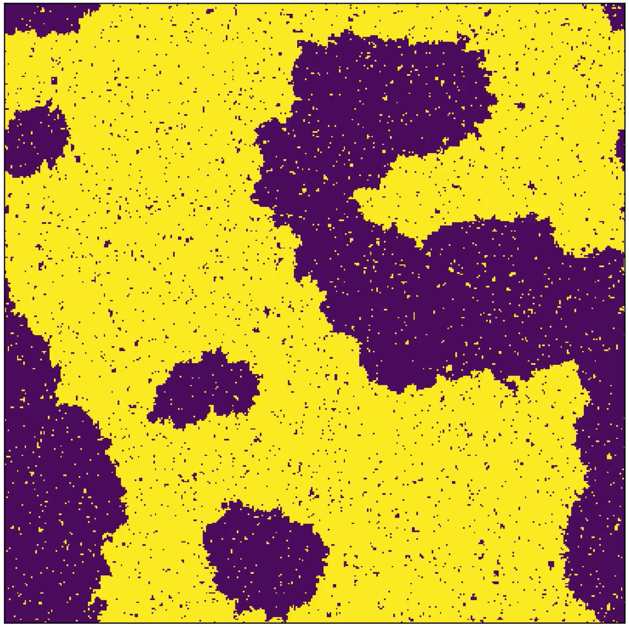
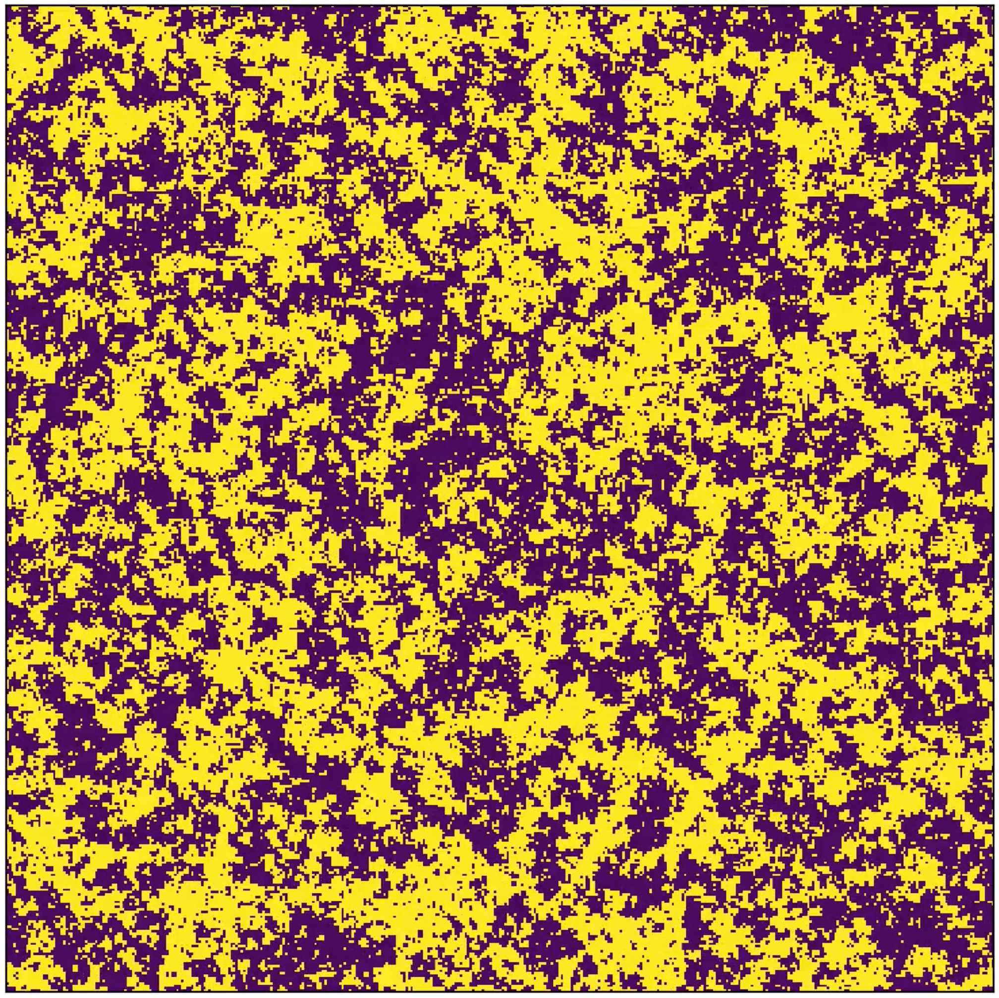
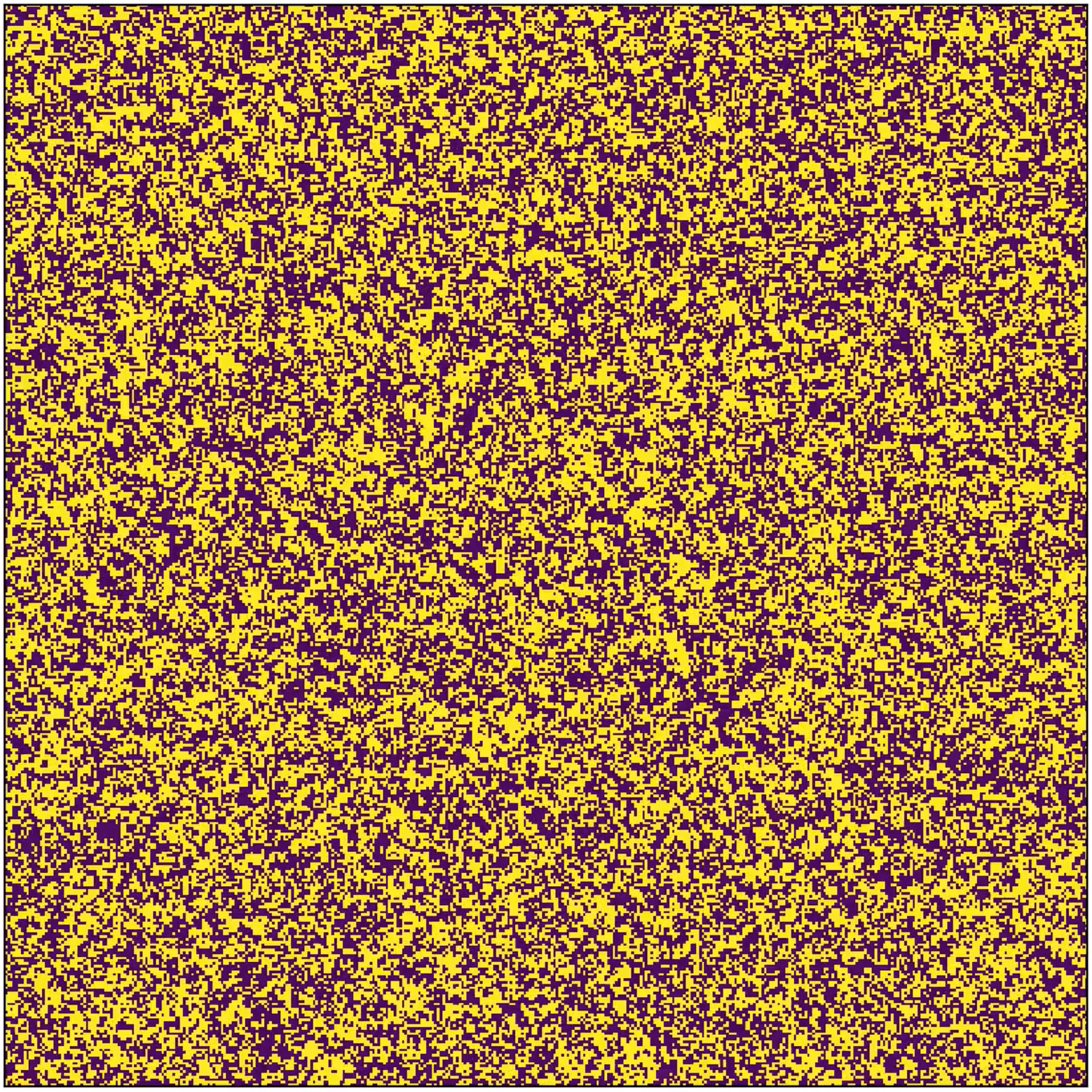
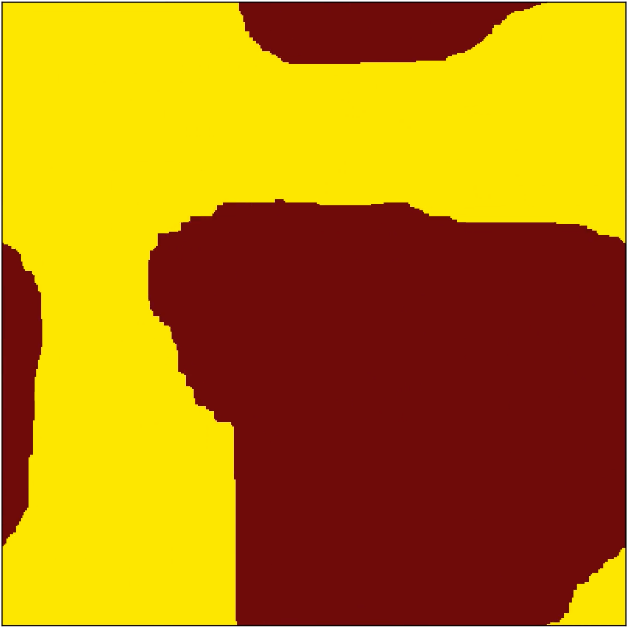
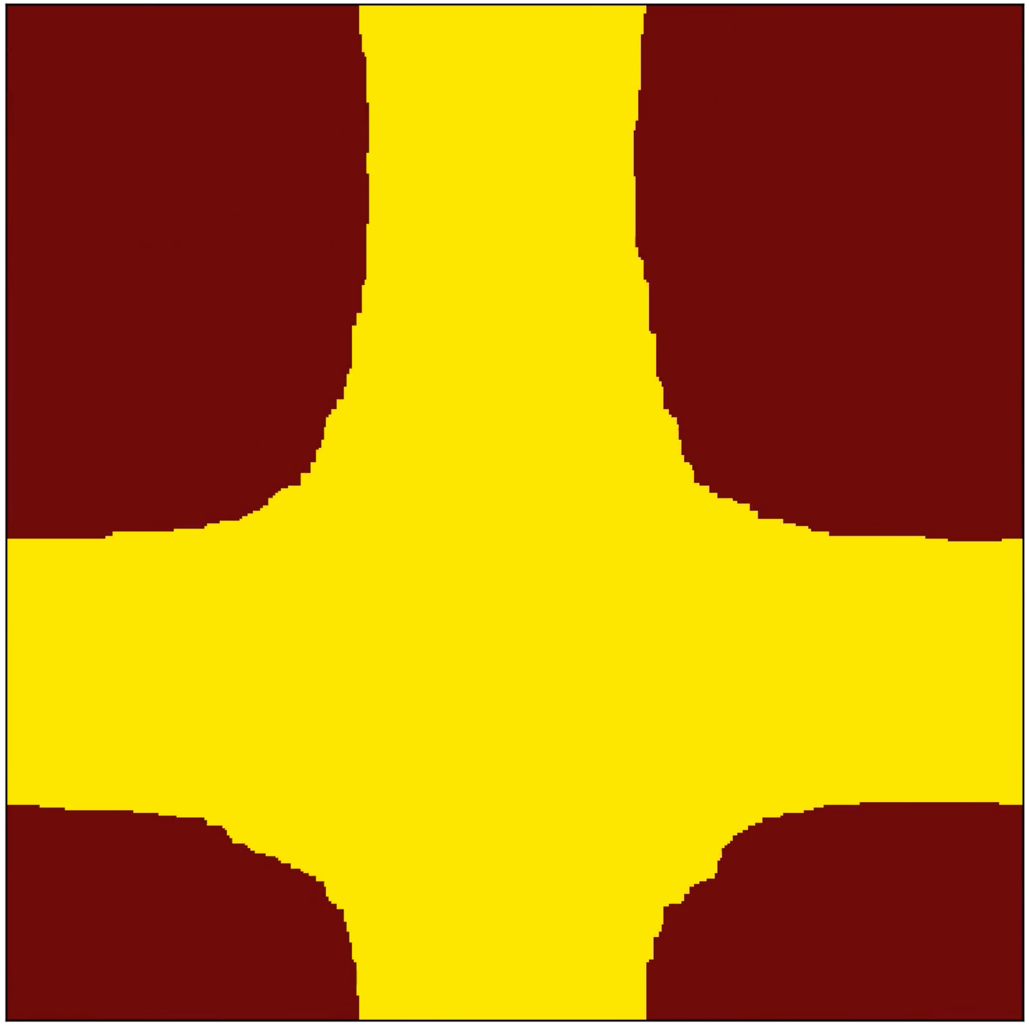
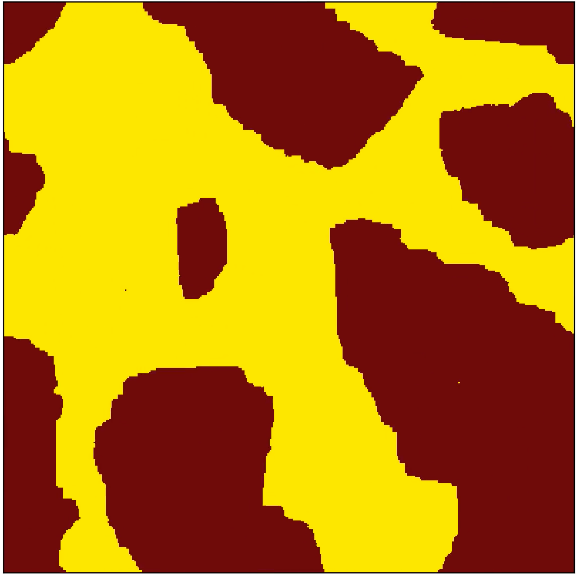
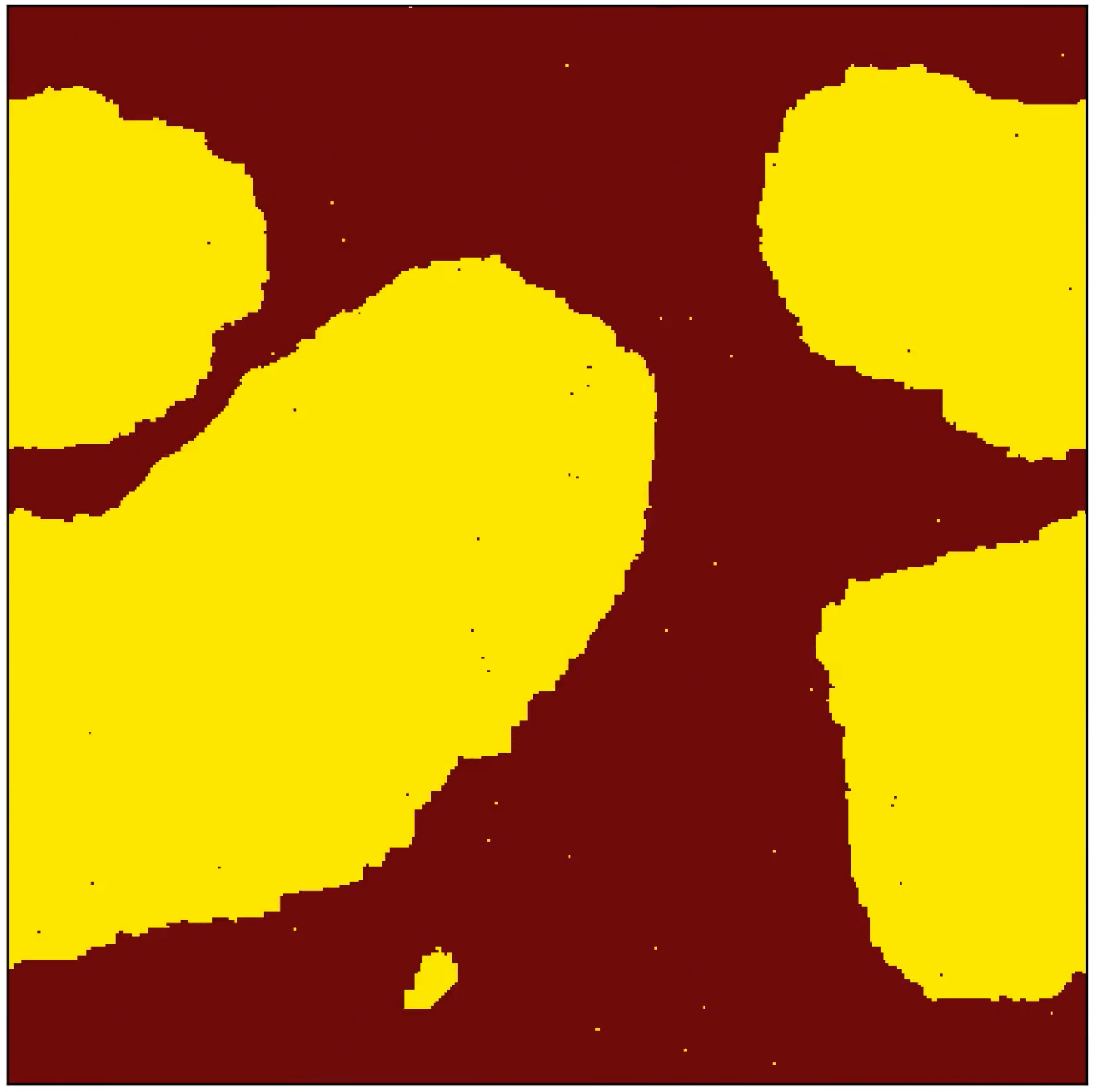
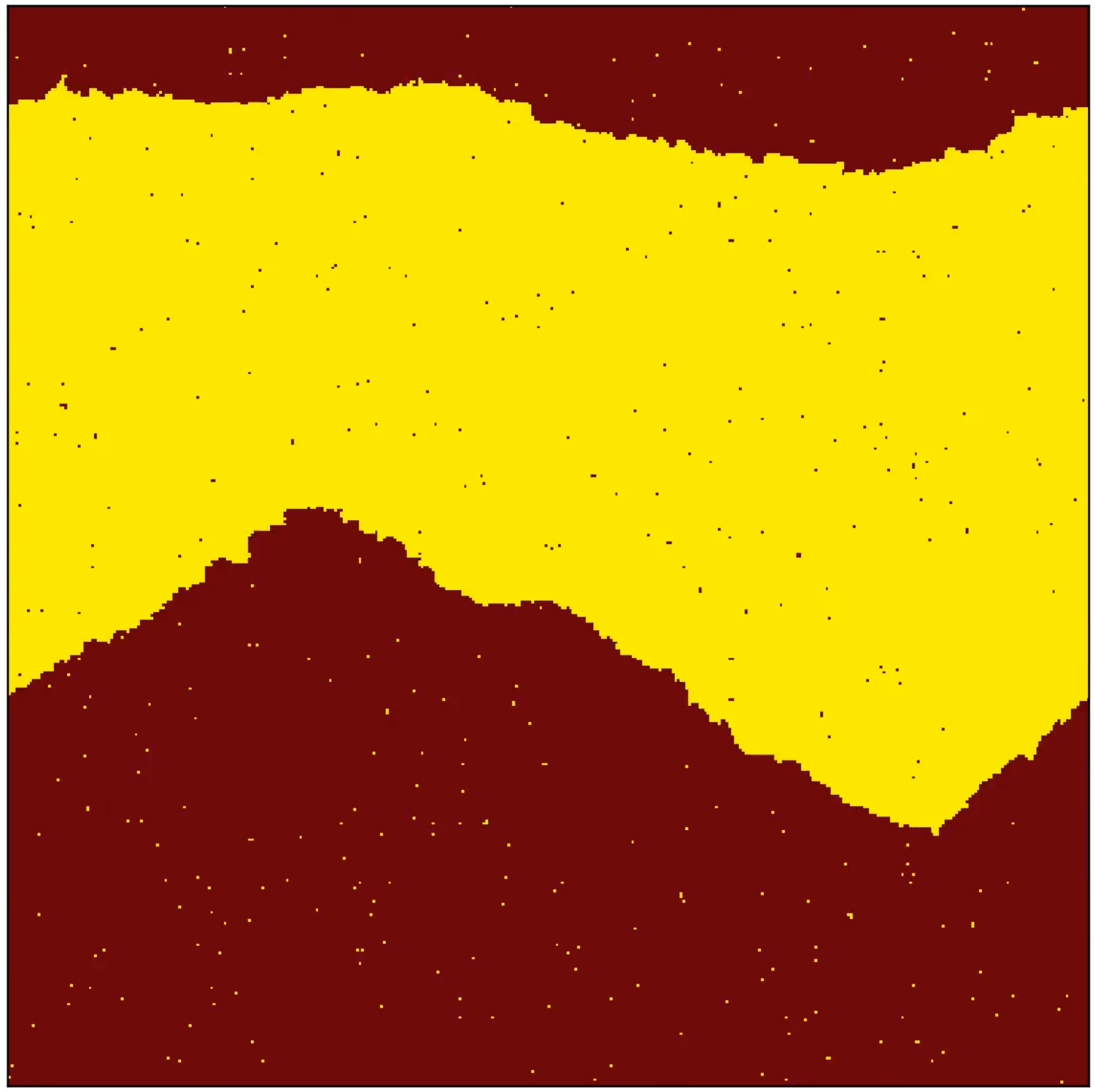
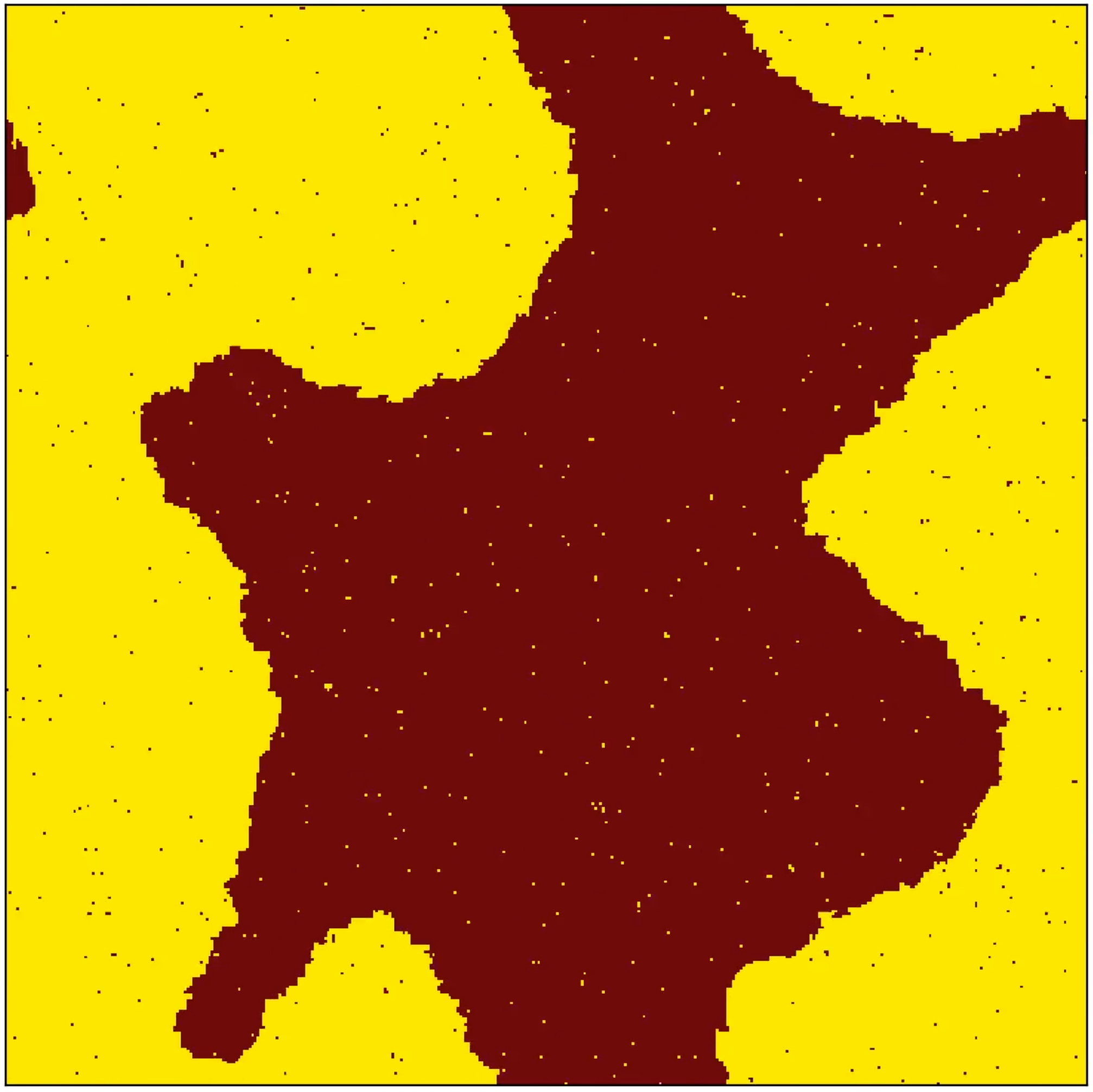
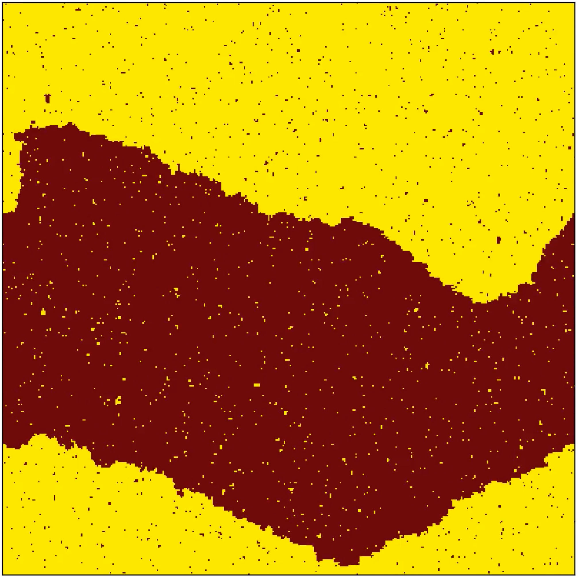
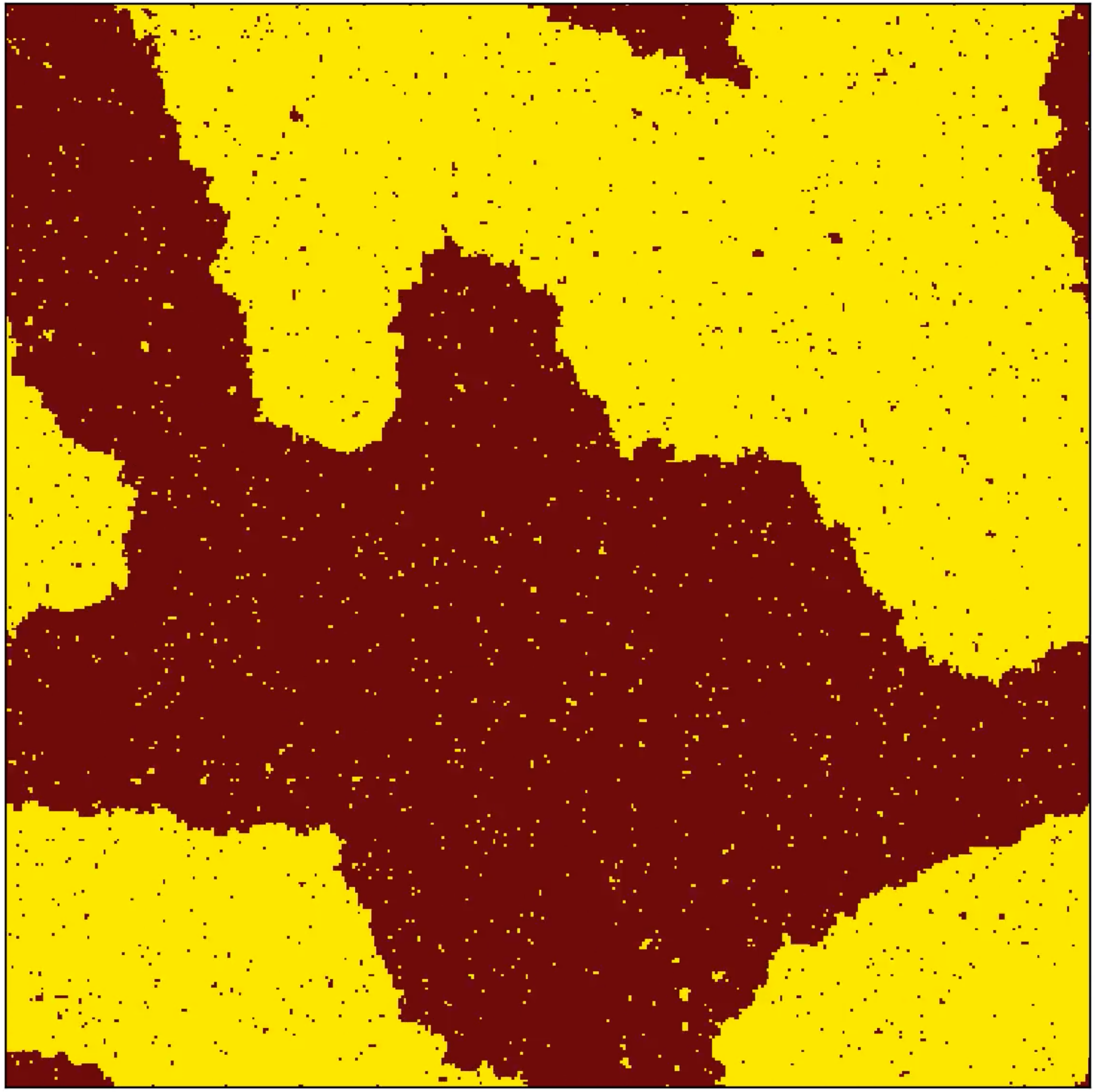
Monte Carlo simulations of a 2D Ising spin model. In both rows of images, the temperature increases from left to right. The images in the lower row were generated by constraining the magnetization to be 50%. Click on every image to start the corresponding animation. Here is the Jupyter notebook that was used to make these animations.
Triangular fractal (click on image to start movie)	Aggregation in 3D (click on image to start movie)
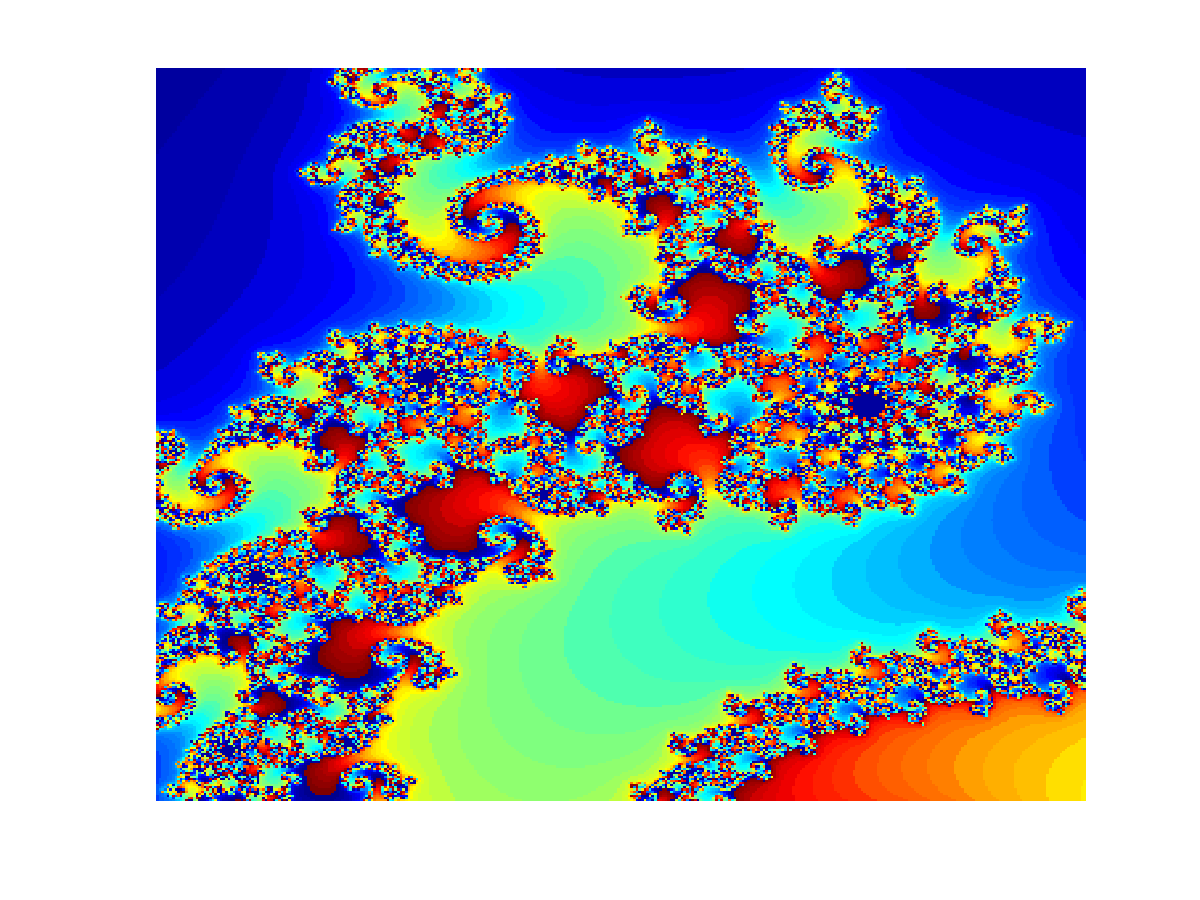
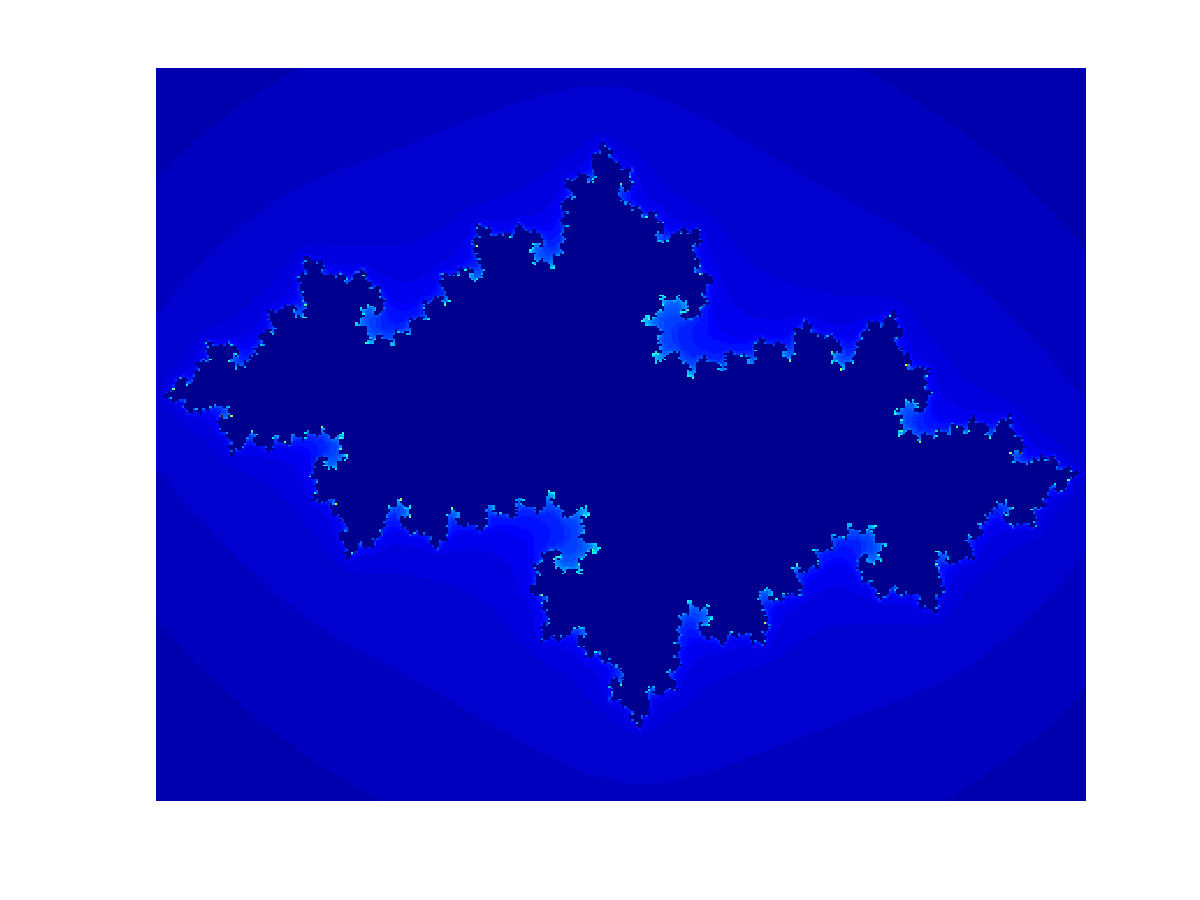
Mandelbrot fractal (click on image to start movie)	Julia set (click on image to start movie)
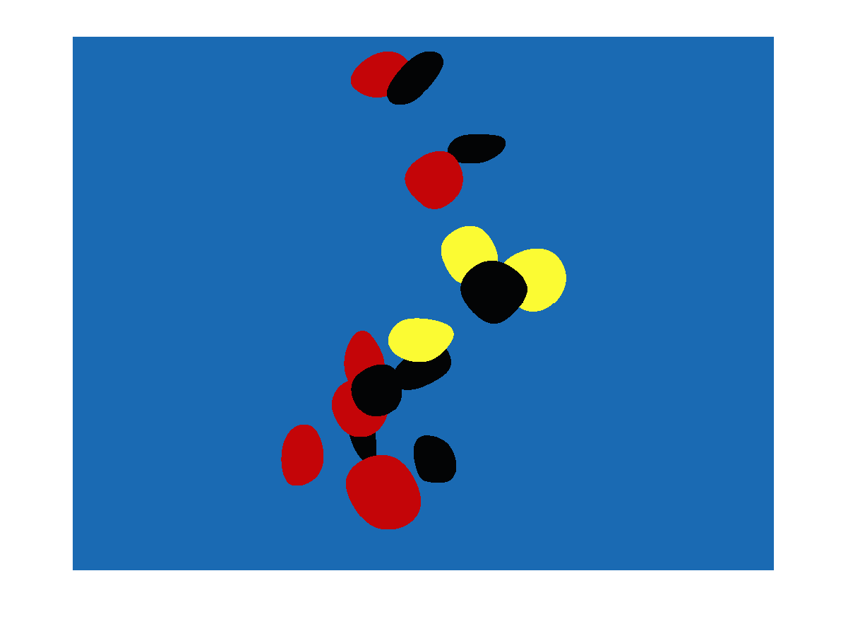
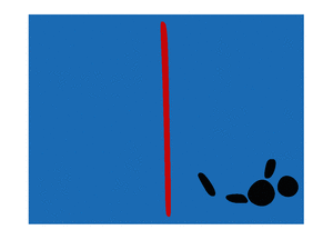In the foot steps of Joan Miro (Higher resolution available: left and right)	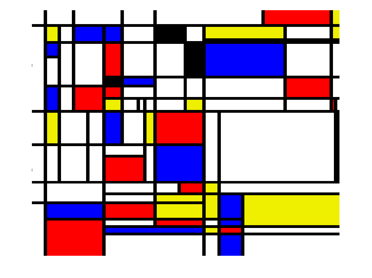In the spirit of Piet Mondrian (higher resolution available)

Landscape evolution model (code written by former EPS109 student Jeff Prancevic) Three movies for different models are available: movie 1, movie 2, and movie 3.

A different landscape evolution model. Click on image to start the animation.

Landscape evolution model rewritten in Python. Click on image to start the animation.

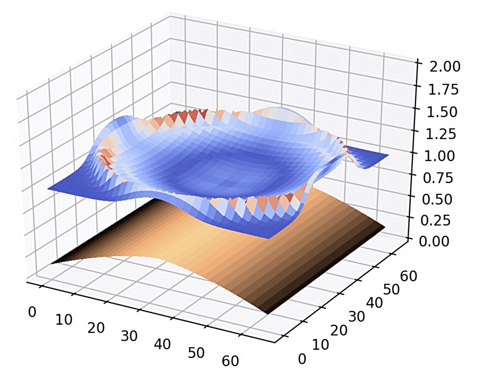
Water wave traveling along a mid-ocean ridge. Numerical solution of the shallow water wave equation. Click on image to start animations 1 or 2 .

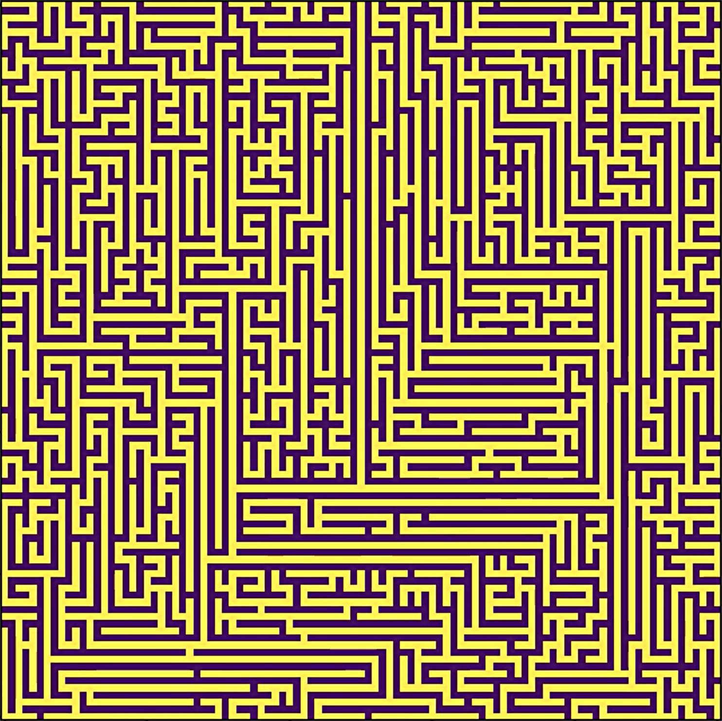
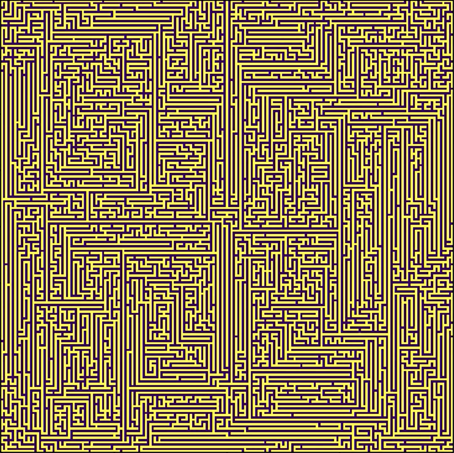
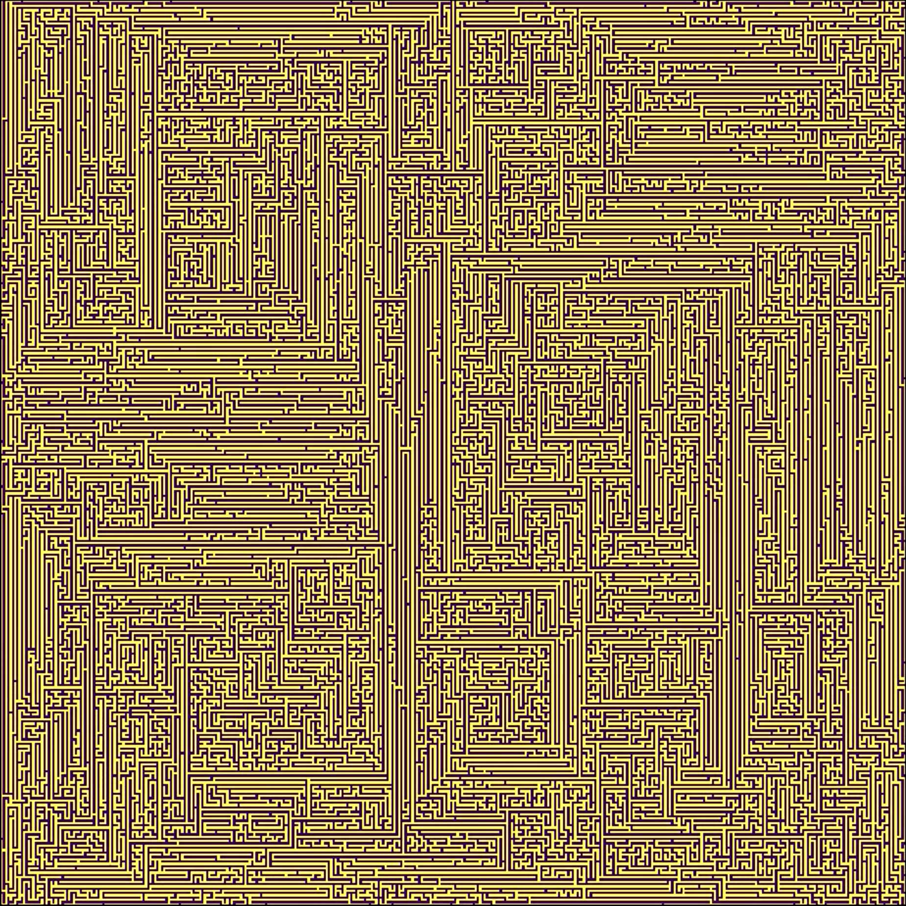
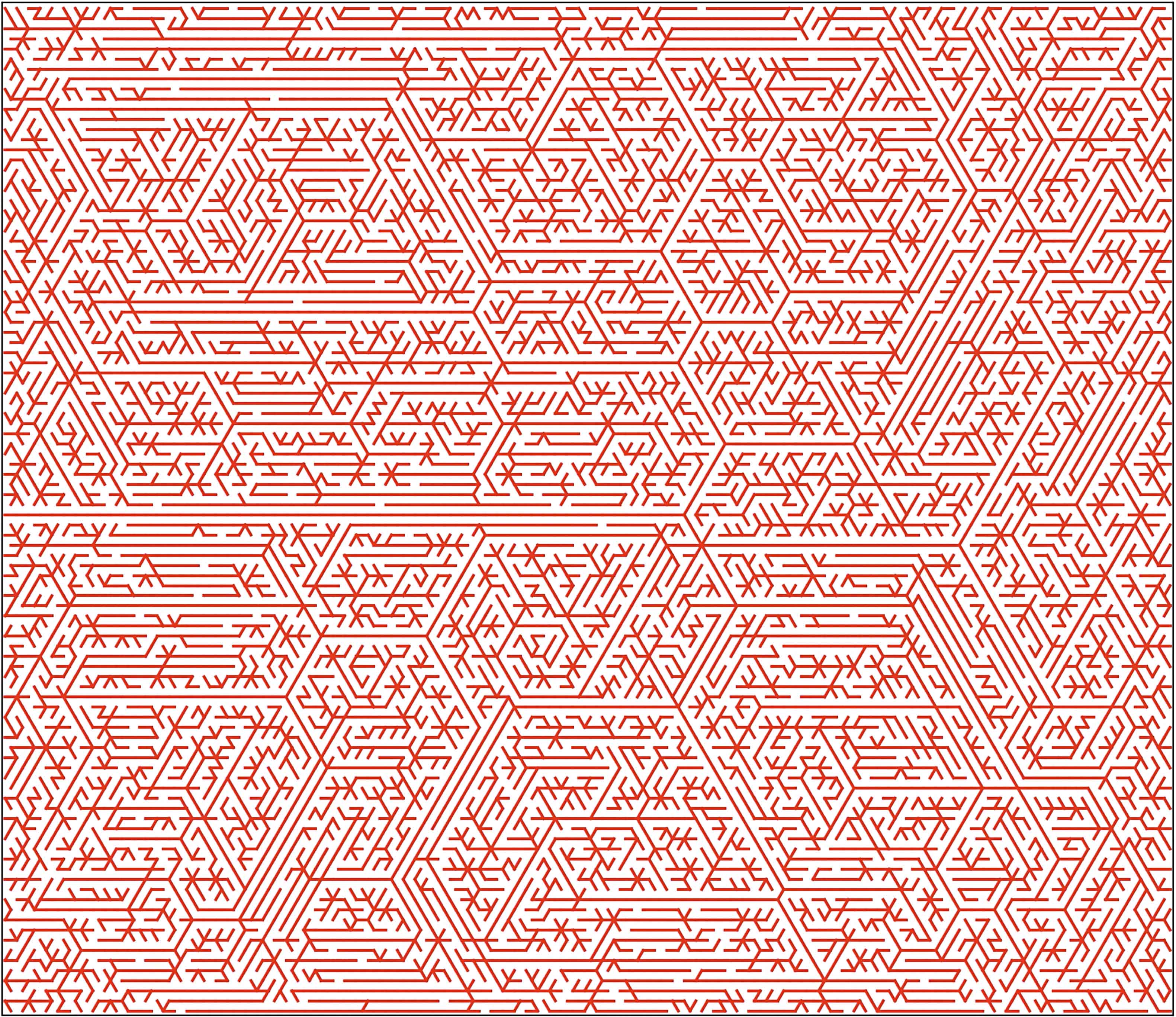
Labyrinths were generated with 101 x 101, 201 x 202, and 401 x 401 resolution and also on a hexagonal grid.

Syllabus:

Date	Lecture topic	Computer lab exercises
Thu 8/27	1: Introduction of course, historical overview, interplay of experiments, theory, and simulation	Lab 1: Matlab as a pocket calculator
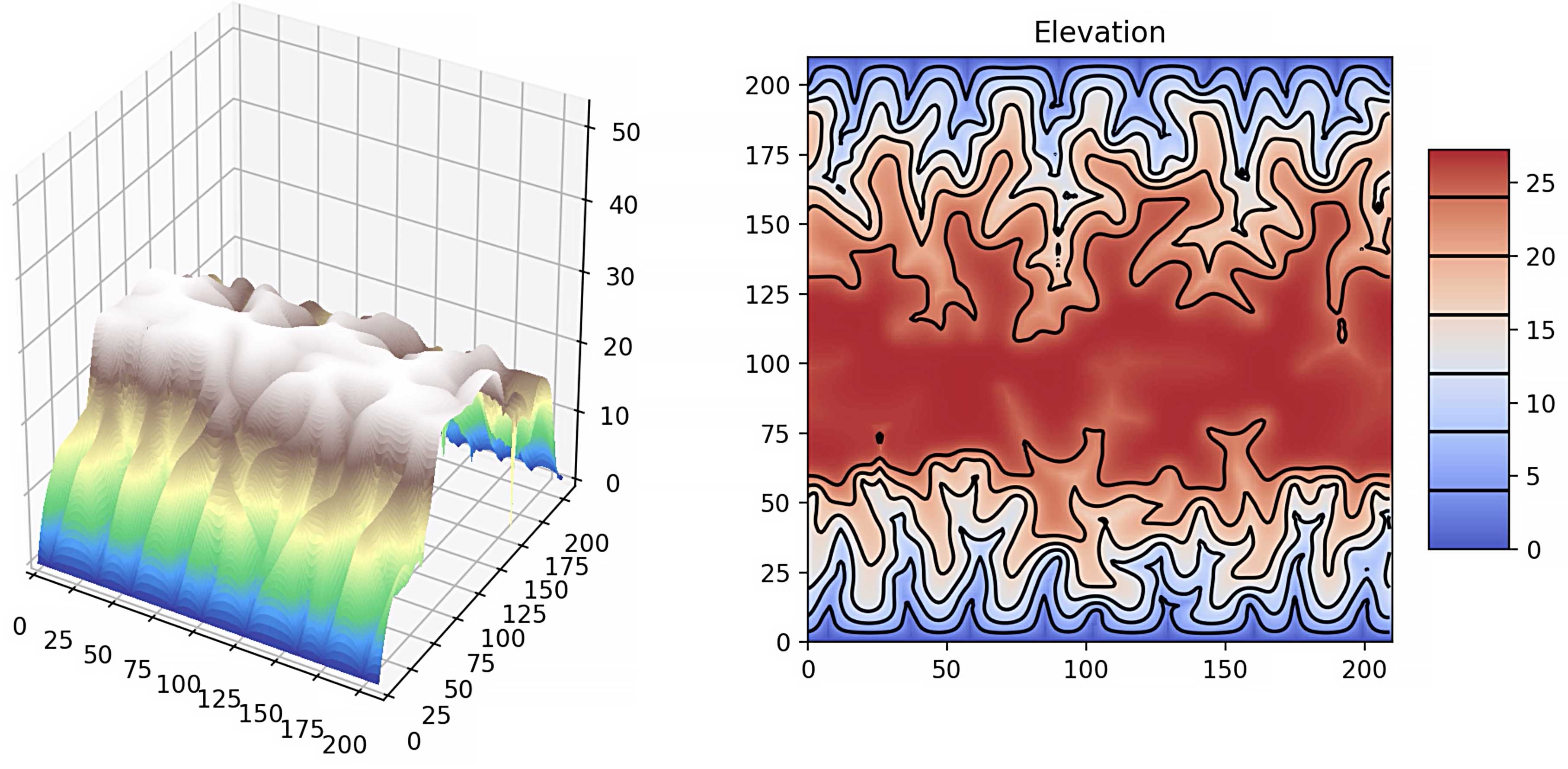
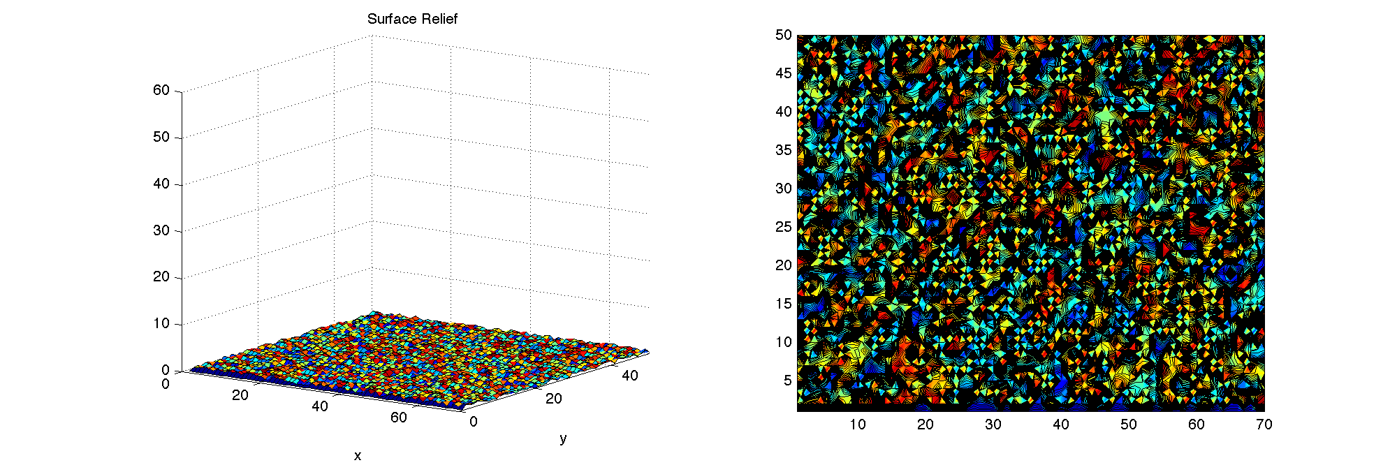
Tue 9/1	2: Fractals in nature, models and computer simulations, fractal dimension and examples in topography and coast line structure	Lab 2: Loops and plots in Matlab
Tue 9/3	3: Mandelbrot set and related fractals
Tue 9/8	4: Random walks and diffusion limited aggregation (DLA), percolation theory	Lab 3: Programming the Mandelbrot and Julia set
Thu 9/10	5: Group discussion on fractals
Tue 9/15	6: Numerical algorithms for finding roots and minima	Lab 4: DLA in 2D on a flat sheet
Thu 9/17	7: Introduction to time independent partial differential equations (PDE), algorithms and stationary state of 1D heat equation
Tue 9/22	8: Methods to find the stationary state of 2D heat equation	Lab 5: Heat equation solver in 2D
Thu 9/24	9: Time dependent PDEs, diffusion equation (heat and chemical diffusion), solution of the 1D heat equation, cooling of a lave dike
Tue 9/29	10: Landscape erosion models	Lab 6: Perron’s erosion model
Thu 10/1	11: Wave equations and numerical solutions
Tue 10/6	12: Shallow water wave equation, tsunamis	Lab 7: 3D water wave simulations
Thu 10/8	Midterm
Tue 10/13	13: Introduction to ordinary differential equations, Euler’s method	Lab 8: Keplerian orbits
Thu 10/15	14: Newton’s law of motion, Keplerian orbits
Tue 10/20	15: Planetary orbits, Hohmann transfers, spacecraft trajectories	Lab 9: Lagrange points
Thu 10/22	16: Runge-Kutta method
Tue 10/27	17: Lagrange points, horseshoe and tadpole orbits of asteroids	Lab 10: Exercise on tadpole and horseshoe orbits
Thu 10/29	18: Strange attractors
Tue 11/3	19: Chaotic dynamical systems and Lyaponov exponents	Lab 11: Roessler attractor
Thu 11/5	20: Simple models for climate change
Tue 11/10	21: Molecular dynamics (MD)	Lab 12: Box model for climate change
Thu 11/12	22: Crystal structures, simulations in periodic boundary conditions
Tue 11/17	23: Many particle simulations	Lab 13: Molecular dynamics I
Thu 11/19	24: Thermodynamic equilibrium, different states of matter
Tue 11/24	25: Introduction to Monte Carlo (MC) simulations	Lab 14: Molecular dynamics II
Thu 11/26	Holiday
Tue 12/1	26: Applications of MC simulations	Lab 15: Comparison of MC and MD
Thu 12/3	27: Curve fitting using the least-squares method, revisions, and exam preparations
Tue 12/8	28: Students present their movie projects, part A	Lab 16: Students present their movie projects, part B

Grade assignment:

The final grade will be calculated using the following percentages:

15% Grades for solving problem sets in weekly computer labs,
35% Grades for homework,
20% One midterm exam taken in class,
30% A final exam taken in class at the end of the semester.


Course description:

109. Computer simulations in Earth and Planetary Sciences (4) Two hours of lecture and two hours of computer lab exercises. Prerequisites: Math 1A or equivalent. Introduction to modern computer simulation methods and their application to selected Earth and Planetary Science problems. In hands-on computer labs, students will learn about numerical algorithms, learn to program and modify provided programs, and display the solution graphically. This is an introductory course and no programming experience is required. Examples include fractals in geophysics, properties of materials at high pressure, celestial mechanics, and diffusion processes in the Earth. Topics range from ordinary and partial differential equations to molecular dynamics and Monte Carlo simulations.

Motivation:

Computer simulations have become an integral part of earth and planetary science (EPS) but students arrive on campus with very different levels of computational skills. This course teaches the fundamental computational methods and their application in EPS. These skills are needed for later course work and research.

Proposed reading list:

(*) C. B. Moler, “Numerical Computing with Matlab”, Society for Industrial and Apllied Mathematics (SIAM) Philadelphia, 2004, QA 297 M625 2004 ENGI, pages 14, 120, 187, 203, available online: http://www.mathworks.com/moler/index.html

Fractals:

(*) H.-O. Peitgen, D. Saupe (ed), The Science of Fractal Images”, Springer Verlag 1988, QA 614 .86 S351 1998 MATH, pages 40, 44, 50, 147, 155,

(*) D. L. Turcotte, “Fractals and Chaos in Geology and Geophysics”, Cambridge, U.K. ; New York : Cambridge University Press, 1997, page 14, 22,45, 59, 69, 71, 91, 97, 149, 201, 235, 299

(*) H.-O. Peigten, H. Jurgens, D. Saupe, “Fractals for the Classroom Part II Complex Systems and Mandelbort Set”, Springer 1992, QA 614 .86 P45 1992 v.2 MATH, pages 27. 58, 127, 199, 304, 318, 381, 401, 420, 446, 453.

(*) B. B. Mandelbrot, “The Fractal Geometry of Nature”, W.H. Freeman and Co. NY 1983,  QA 447 M357 1983 MATH, pages 30, 112,

D.J. Higham, N. J. Highham, “Matlab Guide”. Society for Industrial and Apllied Mathematics (SIAM) Philadelphia, 2000, QA 297 H5217 2000 ENGI, pages 14, 17, 90, , 132, 178, 221, 246.

A. Stanoyevitch, “Introduction to MATLAB with Numercial Preliminaries” Wiley 2004, TA 345 S75 2004 ENGI, pages 177.

J. Feder, “Fractals” Plenuym Press, NY, 1988, QA 447 F371 1998 MATH.

Ordinary Differential Equations, Molecular Dynamics, Solar System Dynamics:

J.H. Mathews, K.D. Fink, “Numerical Methods Using Matlab”, 4th edition, Pearson Education Inc., 2004, QA 297 M39 2004 ENGI, pgaes: 262, 418, 434, 465, 496, 505, 544, 557, 567,

(*) J. B. Marion, S. T. Thornton, “Classical Dynamics of particles and systems”, Saunders College Publishing, Fort Worth Philadelphia.

C.D. Murray, S.F Dermott, “Solar Systems Dynamics”, Cambridge University Press, 1999.

I. De Pater, J.J. Lissauer, “Planetary Science”, Cambridge University Press, 2001.

M. P. Allen, D.J. Tildesley, “Computer Simulations of Liquids”, Oxford University Press.

S. Nakamura, “Numerical Analysis and Graphic Visualization with Matlab” 2nd edition, Prentice Hall PTR 2001, T 385 N34 2002 ENGI, pages 63, 302, 385, 396, 453, 465.

W. J. Palm III, “Introduction to Matlb 6 for Engineers”, McGraw-Hill, 2001, TA 345 P35 2001 ENGI, pages  452.

H. B. Wilson, L. H Turcotte, “Advanced Mathematics and Mechanics Applications Using Matlab”, 2nd edition, CRC Press 1997, TA 354 W55 1997 ENGI, pages: 271, 352, 382.

A.H.Nayfeh, B. Balachandram, “Applied Nonlinear Dynamics, Analytical Computational, and Experimental Maethods”, Wiley, QA 845 N39 1994 ENGI.

E. A. Jackson, “Perspectives of Non-linear Dynamics”, Cambridge University Press, 1989, QA 845 J28 1989 V.1 ENGI

V.S. Anishchenko, V. Astakhov, A. Neiman, T. Vadivasova, L. Schimansky-Geier, “Nonlinear Dynamics of Chaotic and Stochastic Systems” Springer 2007, QA 845 .N667 2007 ENGI, pages 110.

Monte Carlo:

M. H. Kalos, P. A. Whitlock, “Monte Carlo Methods”, John Wiley & Sons, NY.

Partial Differential Equations:

(*) D. L. Turcotte and G. Schubert, “Geodynamics”, Cambridge ; New York : Cambridge University Press, 2002.

X.-S. Yang, “An Introduction to Computational Engineering with Matlab”, Cambridge International Science Publishing, 2006, TA 345 Y36 2006 ENGI, pages 33, 53, 57, 79, 224

W. E. Boyce, R. DiPirma, “Elementary Differential Equations and Boundary Value Problems”, Textbook, John Wiley & Sons, NY.

Climate:

K. Mcguffie, A. Henderson-Sellers, “A Climate modeling Primer”, Wiley 1997, QC 981 M482 1997 EART, page 85

(*) indicates the most relevant books.