Next: Finite Temperature Jastrow Factor
Up: Path Integral Monte Carlo
Previous: Conclusions
Contents
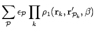
Variational Interaction Terms
The general equations for the variational parameters  in a
parameterized density matrix, from Eq. 3.19, are
in a
parameterized density matrix, from Eq. 3.19, are
 |
(230) |
where
 |
(231) |
and the norm matrix
 |
(232) |
with
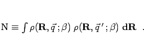 |
(233) |
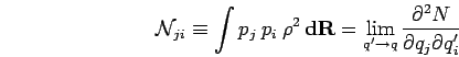
The subscript  in Eq. A.2 indicates that only one
  needs
to be antisymmetric and the identity permutation can be used in the
other. This appendix contains the detailed formulae for
these equations for a parameterized Gaussian density matrix applied to
a Coulomb system.
needs
to be antisymmetric and the identity permutation can be used in the
other. This appendix contains the detailed formulae for
these equations for a parameterized Gaussian density matrix applied to
a Coulomb system.
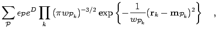
Repeating Eq. 3.56, the parameterized variational density
matrix is an anti-symmetrized product of one-particle density matrices,
where the amplitude  and the widths
  and means
  are the variational parameters. We also dropped
  prefactors
which are the same for the norm matrix and thus cancel out. The
permutation sum is over all permutations of identical particles
(e.g. same spin electrons) and
prefactors
which are the same for the norm matrix and thus cancel out. The
permutation sum is over all permutations of identical particles
(e.g. same spin electrons) and
 is the
permutation signature. The initial conditions are
is the
permutation signature. The initial conditions are  ,
,
 , and
, and  .
.
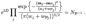
For this ansatz the generator of the norm matrix,
For a periodic system the above equation also is summed over all periodic
simulation cell vectors,  , with
 .
Using this the components of the norm matrix are then:
.
Using this the components of the norm matrix are then:
 |
 |
 |
(236) |
 |
|
![$\displaystyle \sum_{\cal P}\epsilon_{\cal P} \left[
{-2({\bf m}_{i}-{\bf m}_{{\cal P}_i})\over w_{i}+w_{{\cal P}_i}}
\right] N_{{\cal P}}$](img1099.png) |
(237) |
 |
|
![$\displaystyle \sum_{\cal P}\epsilon_{\cal P}
\left({-1\over w_{i}+w_{{\cal P}_i...
... m}_{i}-{\bf m}_{{\cal P}_i})^{2} \over w_{i}+w_{{\cal P}_i}}
\right]N_{\cal P}$](img1101.png) |
(238) |
 |
|
![$\displaystyle \sum_{\cal P}\epsilon_{\cal P} \left[
{2\delta_{j,{\cal P}_i}\sta...
...m}_{{\cal P}_{j}^{-1}}) \over (w_{j}
+w_{{\cal P}_j ^{-1}})}
\right] N_{\cal P}$](img1103.png) |
(239) |
 |
|
![$\displaystyle \sum_{\cal{P}}\epsilon_{\cal{P}} \left[
{\delta_{j,{\cal P}_i}\ov...
... m}_{i}-{\bf m}_{{\cal P}_i})\over w_{i}+w_{{\cal P}_i}}
\right] \!\!N_{\cal P}$](img1105.png) |
|
 |
|
![$\displaystyle \sum_{\cal{P}}\epsilon_{\cal{P}} \left\{
{\delta_{j,{\cal P}_i}\o...
...}} \right]\right.
+{1\over (w_{i}+w_{{\cal P}_i})(w_{j}+w_{{\cal P}_{j}^{-1}})}$](img1107.png) |
|
| |
|
![$\displaystyle \hspace*{.5in} \left.
\left[{3 \over 2}- {({\bf m}_{i}- {\bf m}_{...
...P}_{j}^{-1}})^{2}\over
w_{j}+w_{{\cal P}_{j}^{-1}}}
\right] \right\} N_{\cal P}$](img1108.png) |
(240) |
 |
|
|
|
 |
|
 |
(241) |
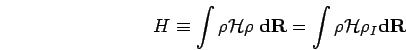
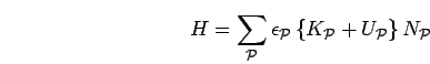
The Hamiltonian for a periodic system of electrons and ions is given by,
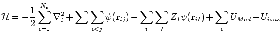 |
(242) |
where the purely ionic terms are,
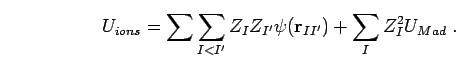 |
(243) |
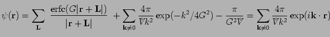
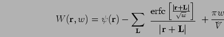
The Ewald potential,  , which includes interactions
with periodic images and incorporates charge neutrality reads,
, which includes interactions
with periodic images and incorporates charge neutrality reads,
where
 is the
periodic cell volume and
is the
periodic cell volume and  an arbitrary constant. The Madelung term in
  is the interaction energy of an electron with it's periodic images and
neutralizing background (e.g.
is the interaction energy of an electron with it's periodic images and
neutralizing background (e.g.
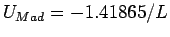 for a simple cubic simulation cell,
the usual case).
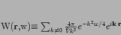
To do the integrals, we represent the Gaussians by their Fourier series
for a simple cubic simulation cell,
the usual case).
To do the integrals, we represent the Gaussians by their Fourier series
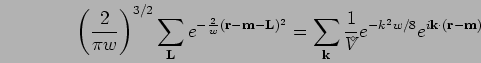 |
(244) |
and in the interaction terms use the Fourier representation for .
This finally gives
 |
(245) |
with
where
 and
and
 .
The interaction integral
.
The interaction integral
 |
(247) |
is symmetric in  when the periodic
cell has inversion symmetry.
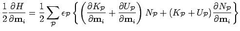
Continuing, the left hand side of Eq. A.1 is
when the periodic
cell has inversion symmetry.
Continuing, the left hand side of Eq. A.1 is
with
where we have used the fact that terms in  and
and
 give the
same contribution under the permutation sum and so combined them.
The derivatives of the interaction integral are,
give the
same contribution under the permutation sum and so combined them.
The derivatives of the interaction integral are,
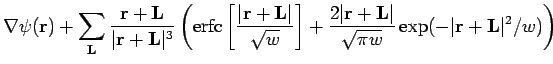
where ![${\bf W}^{[1]}$](img1148.png) and
and ![$W^{[2]}$](img1149.png) denote the derivatives of
denote the derivatives of  with the first
and second argument.
Comparing equation A.18 and Eq. A.15 the interaction
integral may be written as
with the first
and second argument.
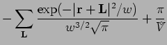
Comparing equation A.18 and Eq. A.15 the interaction
integral may be written as
 |
(255) |
and its derivatives as:
For an isolated system (
 ) and these would
simplify to,
) and these would
simplify to,
At  , the initial derivatives for the variational parameters reduce to
For large numbers of electrons, the computational requirements to
treat all exchange terms increase drastically. Here the approximation
discussed in section
3.7 is used where
the kinetic pair exchange corrections given there are added to the
identity permutation term derived here.
Next: Finite Temperature Jastrow Factor
Up: Path Integral Monte Carlo
Previous: Conclusions
Contents
Burkhard Militzer
2003-01-15

![$\displaystyle \sum_{i}\left[ \frac{3}{w_{i}+w_{{\cal P}i}} -
2\frac{({\bf m}_{i}-{\bf m}_{{\cal P}i})^{2}}{(w_{i}+w_{{\cal P}i})^{2}}\right ]$](img1121.png)


![$\displaystyle \left[-\frac{3}{w_{i}+w_{{\cal P}i}} +
2\frac{({\bf m}_{i}-{\bf m}_{{\cal P}i})^{2}}{(w_{i}+w_{{\cal P}i})^{2}}\right]N_{\cal P}$](img1134.png)
![$\displaystyle \left[
-4\frac{({\bf m}_{i}-{\bf m}_{{\cal P}i})}{w_{i}+w_{{\cal P}i}}\right] N_{\cal P}$](img1136.png)
![$\displaystyle \left[-\frac{6}{(w_{i}+w_{{\cal P}i})^{2}}+
8\frac{({\bf m}_{i}-{\bf m}_{{\cal P}i})^{2}}{(w_{i}+w_{{\cal P}i})^{3}}\right]$](img1138.png)
![$\displaystyle \left[
-8\frac{{\bf m}_{i}-{\bf m}_{{\cal P}i}}{(w_{i}+w_{{\cal P}i})^{2}}\right]\;.$](img1140.png)
![$\displaystyle \frac{2 w_{{\cal P}i}}{w_{i}+w_{{\cal P}i}}
\left[
\sum_{j\neq i}...
...})-\sum_{I}Z_{I}
{\bf W}^{[1]}(\tilde{m}_{i}-{\bf R}_{I},\tilde{w}_{i})
\right]$](img1144.png)
![$\displaystyle \frac{2 w_{{\cal P}i}}{(w_{i}+w_{{\cal P}i})^{2}} \left[
w_{{\cal...
...um_{I} Z_{I} W^{[2]}(\tilde{m}_{i}-
{\bf R}_{I}, \tilde{w}_{i}) \right)
\right.$](img1146.png)
![$\displaystyle \hspace*{-0.05in} + \left.
({\bf m}_{{\cal P}i}-{\bf m}_{i})\cdot...
..._{I}Z_{I}
{\bf W}^{[1]}(\tilde{m}_{i}-{\bf R}_{I},\tilde{w}_{i})\right)
\right]$](img1147.png)
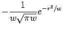
![$\displaystyle \frac{\mbox{erf}\;[r/\sqrt{w}\;]}{ r}$](img1158.png)
![$\displaystyle -\frac{{\bf r}}{r^{3}}\left(
\mbox{erf}\;[r/\sqrt{w}\;]-\frac {2 r}{\sqrt{\pi w}}e^{-r^{2}/w}\right)$](img1159.png)