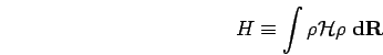
Variational Principle for the Many Body Density Matrix

The Gibbs-Delbruck variational principle for the free energy based on a trial density matrix

$$F\leq \mbox{Tr}[\tilde{\rho}{\mathcal{H}}]+kT\;\mbox{Tr}[\tilde{\rho}\ln\tilde{\rho}]$$ (121)

where

$$\tilde{\rho}=\rho/\mbox{Tr}[\rho]$$ (122)

is well known and convenient for discrete systems (e.g. Hubbard models) but the logarithmic entropy term makes it difficult to apply to continuous systems. Here, we propose a simpler variational principle patterned after the Dirac-Frenkel-McLachlan variational principle used in the time dependent quantum problem (McLachlan, 1964). Consider the quantity

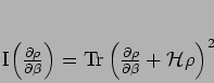$$I\left(\frac{ \partial \rho}{\partial \beta}\right)= \mbox... ... \partial \rho}{\partial \beta} + {\mathcal{H}}\rho\right)^{2}$$ (123)

as a functional of

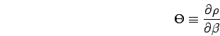$$\Theta\equiv \frac{ \partial \rho}{\partial \beta}$$ (124)

$$I\left(\Theta\right)= \mbox{Tr}\left(\Theta + {\mathcal{H}}\rho\right)^{2}$$ (125)

with $\rho$ fixed. $I\left(\Theta\right)=0$ when $\Theta$ satisfies the Bloch equation, $\Theta=-{\mathcal{H}}\rho$, and is otherwise positive. Varying $I$ with $\Theta$ gives the minimum condition

$$\mbox{Tr}\;\left[ \delta\Theta\left(\Theta +{\mathcal{H}}\rho\right)\right]=0 \quad.$$ (126)

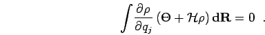
This may be written in a real space basis as

$$\int\int \delta\Theta({\bf R'},{\bf R};\beta) \left[\Theta({... ...\bf R},{\bf R'};\beta) \right] {\bf d}{\bf R}{\bf d}{\bf R'}=0$$ (127)

or, using the symmetry of the density matrix in ${\bf R}$ and ${\bf R'}$,

$$\int\int \delta\Theta({\bf R},{\bf R'};\beta) \left[\Theta({... ...{\bf R'};\beta) \right] {\bf d}{\bf R}{\bf d}{\bf R'}=0 \quad.$$ (128)

Finally, we may consider a variation at some arbitrary, fixed ${\bf R'}$ to get

$$\int \delta\Theta({\bf R},{\bf R'};\beta) \left[\Theta({\bf ... ...{\bf R'};\beta) \right] {\bf d}{\bf R}=0\;\;\forall {\bf R'}.$$ (129)

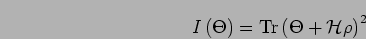
It should be noted that in going from Eq. 3.9 to Eq. 3.10 a density matrix symmetric in ${\bf R}$ and ${\bf R'}$ is assumed, which is a property of the exact density matrix. If the variational ansatz does not manifestly have this invariance Eq. 3.11 minimizes the quantity,

$$\int \left[\Theta({\bf R},{\bf R'};\beta)+{\mathcal{H}}\rho({\bf R},{\bf R'};\beta) \right]^{2} {\bf d}{\bf R}=0 \quad.$$ (130)

This represents the actual variational principle that will be used throughout this work. By construction, it leads to an approximate solution of the Bloch equation, which we propose to derive by parameterizing the density matrix with a set of parameters $q_i$ depending on imaginary time $\beta$ and ${\bf R'}$,

$$\rho({\bf R},{\bf R'};\beta)=\rho({\bf R},q_1,\ldots,q_m) \q... ...ox{where} \quad q_i = q_i({\bf R'};\beta),\quad i = 1,\ldots,m$$ (131)

so

$$\Theta({\bf R},{\bf R'};\beta)=\sum_{i=1}^m \frac{\partial... ...m_{i=1}^m \dot{q}_i \: \frac{\partial \rho}{\partial q_i}\;.$$ (132)

In the imaginary time derivative $\Theta$, only variations in $\dot{q}$ and not ${q}$ are considered since $\rho$ is fixed so,

$$\delta \Theta({\bf R},{\bf R'};\beta) = \sum_{i=1}^m \delta ... ...ta) \: \frac{\partial \rho({\bf R},{q})}{\partial q_i} \quad.$$ (133)

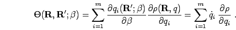
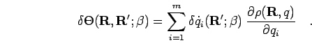
Using this in equation 3.11 gives for each variational parameter, since these are independent,

$$\int \! \frac{\partial \rho}{\partial q_j} \left(\Theta + {\mathcal{H}}\rho \right) {\bf d}{\bf R}= 0\;\;.$$ (134)

This is the imaginary-time equivalent to the approach of Singer and Smith (1986) for an approximate solution of the time dependent Schödinger equation using wave packets (see section 3.3). Introducing the notation

$$p_i \equiv \frac{\partial(\mbox{ln} \rho)}{\partial q_i}$$ (135)

and using Eq. 3.14, the fundamental set of first order differential equations for the dynamics of the variation parameters in imaginary time follows from Eq.. 3.16 as,

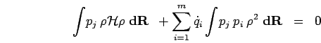$$\int\! p_j \: \rho {\mathcal{H}}\rho\;{\bf d}{\bf R}\:\; + ... ...i \int\! p_j \: p_i \: \rho^2 \; {\bf d}{\bf R} \;\; = \;\; 0$$ (136)

or in matrix form

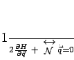$$\frac{1}{2}\frac{\partial H}{\partial \vec{q}}\; + \;\, ... ...\textstyle \leftrightarrow}}{{\mathcal{N}}}\: \dot{\vec{q}}= 0$$ (137)

where

$$H \equiv \int \rho {\mathcal{H}}\rho\;{\bf d}{\bf R}$$ (138)

and the norm matrix

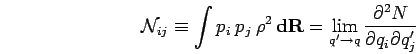$${\mathcal{N}}_{ij}\equiv \int p_i \: p_j \: \rho^2 \, {\bf d... ...im_{q'\to q} \frac{\partial^2 N}{ \partial q_i \partial q'_j}$$ (139)

with

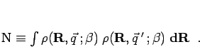$$N \equiv \int \rho({\bf R},\vec{q}\,;\beta) \; \rho({\bf R},\vec{q}\:'\,;\beta)\;{\bf d}{\bf R}\;\;.$$ (140)

The initial conditions follow from the free particle limit of the density matrix at high temperature, $\beta \to 0$,

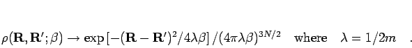$$\rho({\bf R},{\bf R'};\beta)\to \exp\left[ -({\bf R}-{\bf ... ...da\beta)^{3N/2} \quad \mbox{where} \quad \lambda = 1/2m\quad.$$ (141)

Various ansatz forms for $\rho$ may now be used with this approach. After considering the analogy to real time wave packet molecular dynamics, the principle is first applied to the problem of a particle in an external field.