The following example describes the restricted path integral method
and illustrates why it leads to the exact solution in the case that
the nodes are exactly known. It represents a simplified version of the
illustration by Ceperley (1996) that uses the example of the hydrogen
molecule. Here, we talk about the simplest possible problem that has a
node: two free identical particles. For those, the exact nodes are
given by,
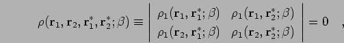 |
(98) |
| (99) |
In this example, we discuss closed paths that end in the reference
point
![]() . In the case of a permutation,
the path must start at
. In the case of a permutation,
the path must start at ![]() , otherwise at
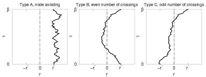
, otherwise at ![]() . One can distinguish
three types of paths as shown in Fig. 2.1,
. One can distinguish
three types of paths as shown in Fig. 2.1,
|
The various kinds of paths have different physical interpretations. In a system of distinguishable particles, no permutations can occur and no nodes exist. Therefore only paths of type A and B contribute. For bosons, one sums over all permutations, nodes are irrelevant and no negative signs come in. For fermions, one has the choice of the direct fermion method or the restricted path method. Both methods are equivalent if the exact nodes are used. In case of the direct method, one considers all permutations with positive and negative signs and does not restrict the path. One sums up contributions from all types including those from type C with a negative sign. For restricted path integrals, one enforces the node, which rules out any permutations in two particle systems. Therefore, there are no negative contributions. Furthermore, the nodal constraint also prevents paths of type B from occurring and one is left with paths of type A, that stay within the half space given by the nodal plane. Essentially, one employs the cancellation of B and C in this method. Both cancel exactly because the flux of the paths is given by the gradient of the density matrix, which is the same on both sides of the node since the derivative is a continuous function. Summarizing, it reads,
The magnitude of the different contributions can also be understood studying the exact solution to the problem stated in Eq. 2.46. For this system of two fermions, it reads,Distinguishable particles: A+B
| (100) |