Nodal Action

In restricted PIMC simulation, one enforces the node by checking the sign of the determinant at each time slice. If it turns out to be negative for a proposed configuration, the move is rejected. The nodes act like an infinite potential barrier. In this method, it is implicitly assumed that the paths do not wander too far between the slices and in particular do not cross a node. This puts an additional lower bound on the number of slices used in a simulation in order to enforce the nodes accurately. By inserting additional slices, one finds that the some paths are rejected on the finer scale, which could not have been detected earlier because they crossed and recrossed the node within the slice. This error can be corrected for by introducing the nodal action $U_N$.

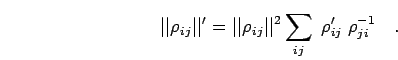
One assumes a flat node between two slices like in the example discussed in the previous section, which is a reasonable approximation for small $\tau$. The difference in action between a system containing a node compared to one without it can be expressed as,

$$e^{-U_N^i} = e^{-(U^i_{\rm rest.}-U^i_{\rm free})} = \frac{... ...-2{\bf d}_i,\tau)} {\rho({\bf r}_{i-1},{\bf r}_i,\tau)} \quad,$$ (101)

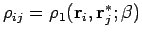
where ${\bf d}_i$ is the distance to the nearest node at the time slice $i$. The image charge is placed at ${\bf r}_i-2{\bf d}_i$. Using the free particle density matrix, the nodal action can be written in terms of the distances to the node at the two slices,

$$e^{-U_N^i} = 1- \exp \, [ \: - \: d_i \, d_{i-1}\:/ \, \lambda \tau \, ] \quad.$$ (102)

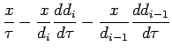
The distance is difficult to calculate but it can be estimated using Newton-Raphson procedure,

$$d_i = \frac{\rho_T({\bf R}_i,{\bf R}^*;\beta)}{\vert\nabla_{\!{\bf R}} \; \rho_T({\bf R}_i,{\bf R}^*;\beta)\vert} \quad.$$ (103)

If $\rho_T$ is given in matrix form $\rho_{ij} = \rho_1({\bf r}_i,{\bf r}^*_j;\beta)$, its derivatives (denoted by $'$) can be calculated efficiently from the cofactor matrix (its transposed inverse) $\rho^{-1}_{ji}$,

$$\vert\vert \rho_{ij} \vert\vert' = \vert\vert \rho_{ij} \vert\vert^2 \sum_{ij} \; \rho_{ij}' \; \rho^{-1}_{ji} \quad.$$ (104)

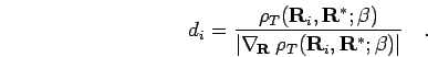
The distance to the node then reads,

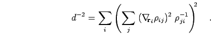$$d^{-2} = \sum_i \left( \sum_j \; ( \nabla_{\!\!{\bf r}_i} \rho_{ij} )^2 \; \rho^{-1}_{ji} \right)^{\!\!2} \quad.$$ (105)

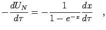
The additional term in the action $U_N$ also leads to a contribution to the internal energy, which can be derived from

$$E_N = - \frac{d U_N}{d \tau} = - \frac{1}{1 - e^{-x}} \frac{dx}{d\tau} \quad,$$ (106)

$$x \equiv \frac{d_{i-1}\;d_i}{\lambda \tau} \quad.$$ (107)

The time derivative of $x$ can be approximated by,

$$-\frac{dx}{d\tau} = \frac{x}{\tau} - \frac{x}{d_i} \frac{d d_i}{d \tau} - \frac{x}{d_{i-1}} \frac{d d_{i-1}}{d \tau}$$ (108)

$$\approx \frac{x}{\tau} \quad.$$ (109)

This approximation omits the change in the distance to the node with imaginary time. It has the advantage that one does not have to compute the derivatives of the distance to the nearest node $d_i$, which would require extra numerical work.

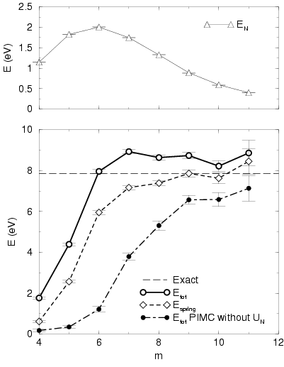
Figure 2.2: Comparison of the internal energy per electron from two simulations, one with nodal action ($\circ$) and one without ($\bullet$), for 16 free particles at $r_s=2.52$ and $T=15\,625\,\rm{K}$ for different number of time slices $2^m$ leading to a time step $\tau^{-1} = 2^{m-6} 10^6\,\rm{K}$. $\triangle$ shows the nodal energy and $\diamond$ denotes the spring kinetic energy given by $E_{tot} - E_N$. The long dashed line shows the exact energy for this finite system. All simulations were $3.2\times 10^6$ steps of level $k=m-3$ long.

The effect of the nodal action $U_N$ is shown in Fig. 2.2, where two simulations, one with it and without it, are compared as a function of time step. In these simulations, $N=16$ spin-polarized free electrons were studied at $T=15\,625\,\rm {K}$ and $r_s=2.520$. The conditions were chosen in correspondence with hydrogen simulations discussed in chapter where 32 protons and 32 electrons in two spin states are studied at a typical density corresponding to $r_s=2.0$. The Fermi temperature for an infinite system (Eq. 2.74) under these conditions is $145\,381\,\rm {K}$. For a system with $N=16$, it becomes $29\,747\,\rm {K}$. The difference is that large because the only 3 $k$-shells are occupied while in Eq. 2.74 sum of k-shells were approximated by an integral. The number of states per k-shell starting from $k=0$ are 1, 6, 12, 8, 6, 24, ...

All hydrogen simulations discussed later are performed with $\tau^{-1}=10^6\,\rm {K}$ (64 slices, $m=6$) or smaller time steps. The required time step can be estimated from the corresponding degeneracy parameter,

$$n \Lambda_\tau^D \equiv n \; ( 4 \pi \lambda \tau )^{D/2} \quad,$$ (110)

which relates the average distance the path travels between the slices,

$$\Delta r \equiv \sqrt{ \left< ({\bf r}_{i+1} - {\bf r}_i)^2 \right> } = \sqrt{ 2 D \pi \lambda \tau }$$ (111)

to the inter-particle spacing. For the above example with $\tau^{-1}=10^6\,\rm {K}$, one finds $n \Lambda_\tau^3 = 0.041$ and $\Delta r = 1.725$, which must be compared to the inter-particle spacing given by $r_s=2.520$. For the example of $N=16$ particles at this degeneracy, Fig. 2.2 predicts that choosing the time step such that $\Delta r / r_s \stackrel{\scriptstyle<}{\scriptscriptstyle\sim}\:0.7$ ( $n \Lambda_\tau^3 \stackrel{\scriptstyle<}{\scriptscriptstyle\sim}\: 0.04$) leads to energies reasonably close to the exact value. To go up to 2048 slices ($m=11$) is only possible for a system of free particles this small. The figure shows clearly that in simulations with the nodal action term, the internal energy converges faster to the exact value of 7.844 eV, the reason being that configurations of paths where the nodal constraints are likely to be violated between the slices are rejected because of the $U_N$ term. However, the graph also shows that the nodal energy is overestimated leading to an internal energy 10% too large. Possible explanations for this discrepancy include the approximations in the way the distance to the node is estimated, the implicit assumption that the nodes are planar within the time interval $\tau$ and the omission of two terms in Eq. 2.99. However, in the limit of small $\tau$ all those approximations do not matter and one should find the above mentioned exact value, which was calculated by a separate MC method in $k$-space. The nodal constraint there is realized by restricting each $k$-point to only one particle. However, the method relies on the exactly known eigenstates of the Hamiltonian.