Next: Distribution of Permutation Cycles
Up: Fermion Nodes
Previous: Nodal Action
Contents
In the previous section, it has been shown how a nodal action can be
used to predict the probability that paths cross the nodes between two
time slices. The procedure has the advantage that it allows to employ
a large time step, which can be crucial for simulation at low
temperature with a high computational demand. However, there exists
still an upper bound on the time step because the assumption of a planar
nodal surface between two slices breaks down. The effects on the
thermodynamic variables calculated from a simulation with too large a
time step are especially drastic in attractive systems like hydrogen.
There, the nodes realize the Pauli exclusion principle, which make
matter stable. If it is not guaranteed the system will inevitably
collapse at some point in time during a simulation as shown by
Theilhaber and Alder (1991).
An example of node violations is shown in Fig. 2.3. All
determinants at a time slice have a positive sign and the predicted
distance to the nodes has a reasonable value greater than 0. However, if
one interpolates the coordinates linearly between two slices and then
calculates the determinant and the distance to the node one finds some
points where the path crosses the node. This could not happen if the nodes
were planar. This analysis shows the break down of the nodal action
procedure described in the previous section for too large time
steps. In a simulation of hydrogen, one finds that the pressure
becomes unphysically low and even negative. Simultaneously, the system
partially collapses.
Fig. 2.3 also reveals ways to improve the nodal action. One
possibility is to study the classical path that connects the two
slices  and
and  in order to predict violations of the nodal
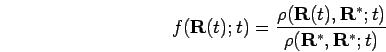
surfaces. We propose to use the function,
in order to predict violations of the nodal
surfaces. We propose to use the function,
 |
(112) |
and to determine its value and its gradient at the two slices. Those
are fit a third order polynomial and it will be checked if it goes
through zero. The reason for dividing by the term
 is that the magnitude of the density matrix
changes considerably even with a small time interval. Checking for node
violations on the classical path gives rise to an additional
restriction for a proposed configuration. In order to derive a nodal
action one needs to study an ensemble of the paths. Due to the lack of
analytical solutions of the diffusion equation for this problem we
suggest to use a set of randomly sampled semi-classical paths,
is that the magnitude of the density matrix
changes considerably even with a small time interval. Checking for node
violations on the classical path gives rise to an additional
restriction for a proposed configuration. In order to derive a nodal
action one needs to study an ensemble of the paths. Due to the lack of
analytical solutions of the diffusion equation for this problem we
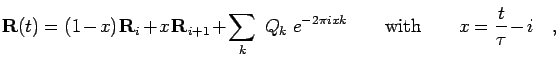
suggest to use a set of randomly sampled semi-classical paths,
 |
(113) |
where  are
are  dimensional normal-mode vectors that have a
Gaussian distribution. The simplest way is to use only the first mode and
to determine the width of the Gaussian from the free particle density
matrix. Practically, one would sample a number , constructed the
corresponding semi-classical paths, perform the fit of
dimensional normal-mode vectors that have a
Gaussian distribution. The simplest way is to use only the first mode and
to determine the width of the Gaussian from the free particle density
matrix. Practically, one would sample a number , constructed the
corresponding semi-classical paths, perform the fit of  to the
polynomial along each paths and check if the node would be crossed.
The fraction of node avoiding paths would then be used in a metropolis
rejection step. This analysis does predict some of the node violations
that could not be detected with previous method. However, a detailed
analysis if it actually improves the efficiency compare to a
simulation with a smaller time step remains to be done.
to the
polynomial along each paths and check if the node would be crossed.
The fraction of node avoiding paths would then be used in a metropolis
rejection step. This analysis does predict some of the node violations
that could not be detected with previous method. However, a detailed
analysis if it actually improves the efficiency compare to a
simulation with a smaller time step remains to be done.
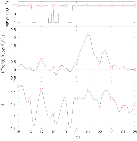
Figure 2.3:
Demonstration of violations of the nodal surfaces for one configuration of
a hydrogen simulation with too large a time step. The  correspond to the time slice, at which the sign of the trial density
matrix is checked. The solid lines display same properties on a
classical path connecting the slices. The middle graphs shows the
trial density matrix
correspond to the time slice, at which the sign of the trial density
matrix is checked. The solid lines display same properties on a
classical path connecting the slices. The middle graphs shows the
trial density matrix
 divided by
 vs. imaginary time
  . The upper graph exhibits
sign of
. The upper graph exhibits
sign of  and in the lower graph, the distance to the node from
Eq. 2.94. The sign of this distance indicates, which side of
the node the paths is on. The classical paths exhibits four node
crossings the could not be predict using the nodal action from
Eq. 2.93. This fact as well the middle graph demonstrates
the nodes are not sufficiently planar in the time interval
and in the lower graph, the distance to the node from
Eq. 2.94. The sign of this distance indicates, which side of
the node the paths is on. The classical paths exhibits four node
crossings the could not be predict using the nodal action from
Eq. 2.93. This fact as well the middle graph demonstrates
the nodes are not sufficiently planar in the time interval  .
.
|
|
Next: Distribution of Permutation Cycles
Up: Fermion Nodes
Previous: Nodal Action
Contents
Burkhard Militzer
2003-01-15