Cellular Automata have the advantage of modeling the traffic flow on the
microscopic scale of individual vehicles and allow the study of large systems
due to a simple type of dynamics. A one-dimensional
model with periodic boundary conditions representing a single lane
freeway was introduced
by Nagel el al. [8, 9] and later slightly modified in [7].
The sites of the array of length L
can be occupied by a vehicle with velocity between zero and ![]() or
be empty. The system is updated in each time step performing the following
steps:
or
be empty. The system is updated in each time step performing the following
steps:

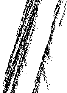
Figure 4: Space-time plot of a traffic jam in the cellular automata
model by Nagel el al. [7]. The horizontal direction is space and
the vertical time. Only the position of cars in jams are shown.
This model has been studied intensively using parallel computers, in
particular, the lifetime of emerging traffic jams such as shown in
Fig. 4. It was shown that the probability distribution as a function
of lifetime follows a power law,
![]()
This exponent is very close to ![]() , which is
the first return-time exponent for a one-dimensional
random walk. This hypothesis was pursued by studying
the probability distribution P(n,t) of a
jam of size n at time t analytically. The time-dependence
of the this distribution is given by,
, which is
the first return-time exponent for a one-dimensional
random walk. This hypothesis was pursued by studying
the probability distribution P(n,t) of a
jam of size n at time t analytically. The time-dependence
of the this distribution is given by,
![]()
This equation describes the growing and shrinking
of a jam, where ![]() and
and ![]() are density dependent parameters
for the rate of cars driving in and out of the jam. From this equation, the
are density dependent parameters
for the rate of cars driving in and out of the jam. From this equation, the

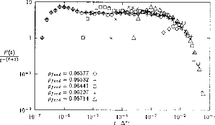
Figure 5:
Data collapse for the lifetime distribution of jams
in the cellular automata
model by Nagel el al. [7].
analogy to a one-dimensional random walk becomes clear. A jam starts
at size n=1 at particular time. It grows, then
shrinks and finally disappears if n is equal to one at a later time.
This is the reason why the life time of a jam can be related to
first return-time of one-dimensional random walk.
Going to the continuum limit in Eq. 6, it can be shown that P
follows a scaling function,
![]()
near the critical point with critical density ![]() .
. ![]() is defined
as
is defined
as ![]() .
In the case of
.
In the case of ![]() , it follows exactly
, it follows exactly ![]() and
and
![]() .
For the numerical results for
.
For the numerical results for ![]() , a data collapse was performed using
, a data collapse was performed using
![]() (Fig. 5). It was found,
(Fig. 5). It was found,
![]()
which agrees with prediction from the random walk model.