Momentum Distribution

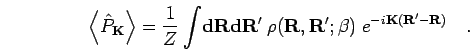
In the path integral formalism, the momentum distribution can be derived by projecting out a many particle state with momentum $\mathbf{K}$. The projection operator is given by,

$$\hat{P}_\mathbf{K} = \left\vert \psi_\mathbf{K}\right> \left< \psi_\mathbf{K}\right\vert$$ (211)

$$= \int \! {\bf d}{\bf R}{\bf d}{\bf R}' \; \left\vert {\bf R}\right> \; e^{-i\mathbf{K}({\bf R}-{\bf R}')} \; \left< {\bf R}' \right\vert \quad.$$ (212)

Applying it to the thermal density matrix using Eq. 2.7 leads to

$$\left< \hat{P}_\mathbf{K}\right> = \frac{1}{Z} \int \! {\bf... ...,{\bf R}';\beta) \; e^{-i \mathbf{K}({\bf R}'-{\bf R})} \quad.$$ (213)

To find the single particle momentum distribution, one averages over the momentum of all particles except the first, which is equivalent to performing the integrals ${\bf d}\mathbf{k}_2 \ldots {\bf d}\mathbf{k}_N$. Including an extra normalization factor of $(2 \pi)^{-ND}$, this leads to the single particle momentum distribution,

$$n(\mathbf{k}) = (2 \pi)^{-3} \int {\bf d}{\bf r}_1 {\bf d}{\... ...k}({\bf r}'_1-{\bf r}_1)} \; \rho^{[1]}({\bf r}_1,{\bf r}_1'),$$ (214)

where $\rho^{[1]}({\bf r}_1,{\bf r}_1')$ is the one-particle reduced density matrix defined in Eq. 5.1. The normalizations are given by $\int \! {\bf d}{\bf r}\, \rho^{[1]}({\bf r},{\bf r}) = {V^{\!\!\!\!\!\!\:^\diamond}}$ and $\int \! {\bf d}\mathbf{k} \, n(\mathbf{k}) = 1$. For isentropic homogeneous systems, the one-particle reduced density matrix is only a function of $\vert{\bf r}-{\bf r}'\vert$, which allows one to introduce the function $n(\vert{\bf r}-{\bf r}'\vert)\equiv\rho^{[1]}({\bf r},{\bf r}')$ with $n(0)=1$. It represents the distribution function of the separation of open ends in a PIMC simulation with one open path.

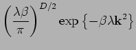
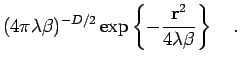
Classical particles exhibit the Maxwellian momentum distribution. Therefore, the single particle density matrix is a Gaussian,

$$n(\mathbf{k}) = \left( \frac{\lambda \beta}{\pi} \right)^{D/2} \exp \left\{-\beta \lambda \mathbf{k}^2\right\}$$ (215)

$$n({\bf r}) = (4 \pi \lambda \beta)^{-D/2} \exp \left\{ -\frac{{\bf r}^2}{4 \lambda \beta }\right\} \quad.$$ (216)

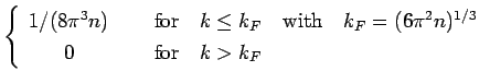
For an ideal Fermi gas at $T=0$, the momentum distribution is a Fermi function,

$$n(\mathbf{k}) = \left\{ \begin{array}{cl} 1/(8 \pi^3 n) & {~~~~\rm {for}}~~~ k\le... ...F = (6 \pi^2 n)^{1/3}\\ 0 & {~~~~\rm {for}}~~~ k > k_F\quad \end{array}\right.$$ (217)

$$n({\bf r}) = 3/x^3 \left[ \sin \, x - x \, \cos \, x \right] ~~~~~~~~~~~~~{\rm {with}}~~~ x = r k_F \quad.$$ (218)

The single particle density matrix $n(r)$ is proportional to the spherical Bessel function $j_1(x)$, which oscillates around zero. In the PIMC simulations, $n(r)$ can be obtained in form of a histogram, in which the separations of the open ends weighted with the sign of the permutation are entered. At separations $r$ where it is negative, odd permutations leading negative contributions must outweigh even permutations making positive contributions. $\vert j_1(x)\vert$ decays slowly as $r^{-2}$, which requires macroscopic exchange cycles to occur. Those are solely a consequence of the discontinuity of $n(k)$ at $k=k_F$.

Before we discuss results from PIMC simulation of interacting systems we will examine the scaling behavior of the off-diagonal sampling method. In order to study a certain number of oscillations in $n(r)$, one can make a simple estimation of how many particles are required. For this purpose, we neglect the fact that Eq. 5.11 was derived in thermodynamic limit, $N \to \infty$. In a simulation using a 3D box of size $L$, one can directly measure $n(r)$ up to $\frac{L}{2}$ and indirectly up to $\frac{L}{2}\sqrt{3}$. This leads to the estimates for the required number of particles given in Tab. 5.1.

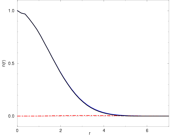
Figure 5.2: $n(r)$ for systems of 33 spin-parallel electrons at $T=125\,000\,{\rm K}$ and $r_s=4.0$ ( $T_F=57\,694\rm K$) (solid line). At this temperature, fermionic effects are only a small correction to the classical behavior. Therefore negative contributions (dash-dotted line) are negligible and the sum of the positive contributions (dotted line) are almost identical to the full $n(r)$. We also found that the repulsive interactions do not lead to significant modification to the non-interacting case given by the Gaussian function in Eq. 5.9.

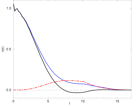
Figure 5.3: $n(r)$ from the system shown in Fig. 5.2 but here for a significantly lower temperature of $T=15\,625\,{\rm K}$, where fermionic effects dominate ( $T_F=57\,694\rm K$). This leads to negative regions in $n(r)$, as expected from the zero temperature limit given by Eq. 5.11. In these regions, odd permutations from exchange cycles with an even number of particles dominate. The functions decrease rapidly at $r=L/2=10.3$ as a result of finite size effects because the minimum image method is applied.

Figure 5.4: $n(r) r^2$ from Fig. 5.2 using the same line styles. The extra $r^2$ factor emphasizes the small fermionic effects that lead to some negative contributions.

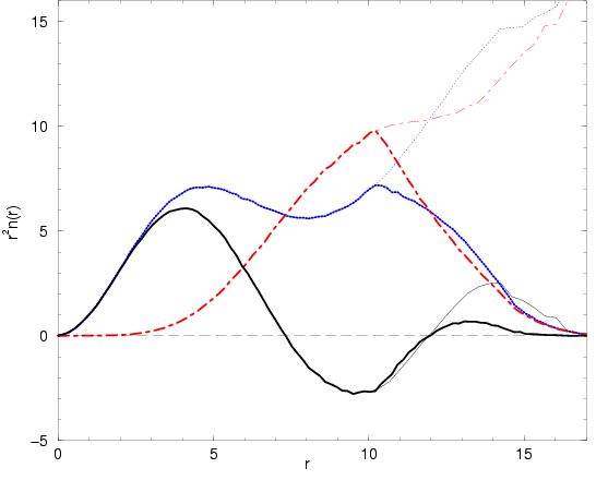
Figure 5.5: $n(r) r^2$ from Fig. 5.3 (thick lines). It shows the oscillating behavior of n=$n(r)$ in fermionic systems (Eq. 5.11). One finds 3 zeros as expected for free particles (see table 5.1). The thin lines show finite size corrections for $r>L/2=10.3$.

Figure 5.6: Momentum distribution $n(k)$ ($\circ$) for a finite system of 33 spin-parallel electrons at $T=125\,000\,{\rm K}$ and $r_s=4.0$ ( $T_F=57\,694\rm K$) also studied in Fig. 5.2. The $\Box$ symbols show the momentum distribution for a finite system of non-interacting fermions under these conditions and the $\Diamond$ display the Maxwell-Boltzmann distribution.

Figure 5.7: Momentum distribution $n(k)$ as in Fig. 5.6 but for a lower temperature of $15\,625\,{\rm K}$. This leads to a degenerate Fermi gas described by a Fermi-Dirac distribution, which is also shown for a system of 33 non-interacting fermions at this $T$ ($\Box$) and at zero temperature (solid line). The difference to the Maxwell-Boltzmann distribution ($\Diamond$) is substantial.

Table 5.1: Minimal number of particles $N$ required to observe the $i$th zero in the single particle density matrix

$i$	$x=r k_F$	$N(\frac{L}{2})$	$N(\frac{L}{2}\sqrt{3})$
1	4.493	12.2	2.4
2	7.725	62.3	12.0
3	10.904	175.1	33.7
4	14.067	376.0	72.4

From this table, one can quickly realize that the computational demand grows rapidly with the number of zeros $i$ because $N \propto i^3$ and CPU time $\propto N^3\propto i^6$. Furthermore, it should be noted that one needs to go to sufficiently low temperatures to observe the fermionic effects and that the CPU time scales linearly with the number of time slices. Additionally, positive and negative contributions cancel, which leads to fluctuations in the observables. The fluctuation do not increase as rapidly as for the direct fermion method (see section 2.6.5) since we still use a nodal restriction but one needs converged results from all cycle lengths, which becomes increasingly difficult at low temperature. A detailed analysis of the scaling behavior with temperature remains to be done.

As a first application of the off-diagonal density matrix sampling method, we chose to study the electron gas because of its simplicity. The method can be easily extended to hydrogen or spin-polarized hydrogen. We looked at a system of 33 closed shell spin-parallel electrons at a density of $r_s=4.0$ ( $T_F=57\,694\rm K$) and selected the two temperatures $125\,000$ and $15\,625\,{\rm K}$ that represent the classical case at high temperature and, respectively, the degenerate electron gas at low temperature. For $125\,000\,{\rm K}$, the observed reduced density matrix $n(r)$ in Fig. 5.2 is in good approximation the classical Gaussian function. Due to the high temperature, permutations are relatively rare. Their contribution can be seen best in Fig. 5.4 where $r^2n(r)$ is shown. Since we multiplied by the volume element $\propto r^2$, the graph can be interpreted as the probability of finding the two ends of the open path separated by $r$. The corresponding momentum distribution $n(k)$ in Fig. 5.6 was calculated directly from MC average,

$$n(\mathbf{k}) \propto \left< e^{i \mathbf{k}({\bf r}-{\bf r}')} \right> \quad,$$ (219)

rather then using a Fourier transform of $n({\bf r})$, which would have required an extrapolation for large $r$ or to store $n({\bf r})$ on a 3D grid because the spherical symmetry is broken by the cubic simulation box. The observed momentum distribution lies between the Maxwell-Boltzmann distribution and the Fermi distribution for the corresponding non-interacting finite system. All three curves are rather close together because the simulation is performed in a classical regime. The deviations of the PIMC result from the free Fermi distribution show the effect of the repulsive interactions between the electrons, which leads to a depletion of the occupation probability at small $k$ values.

This effect is also present in the low temperature results at $15\,625\,{\rm K}$ where one finds a degenerate electrons gas. The momentum distribution in Fig. 5.7 is a Fermi function rather than a Maxwell-Boltzmann distribution, which can reach arbitrarily higher occupation for $k=0$ because it is not limited by the Pauli exclusion principle. The solid line denotes the ideal Fermi gas at $T=0$ given by Eq. 5.10. Thermal excitations as well as the Coulomb interaction lead to the population of momentum states above the ideal Fermi momentum. For interacting systems at $T=0$, a discontinuity in the momentum distribution is still present but some states are pushed to higher $k$-values (Ortiz and Ballone, 1994). The comparison with the ideal Fermi gas at $T=0$ gives an estimate for the thermal excitations at this temperature. The degree of degeneracy is rather high, which has a significant consequence for the reduced density matrix shown in Figs. 5.3 and 5.5. The latter graph shows how positive contributions dominate at small separations $r$. Then the function goes through zero and even permutations dominate. After that, it becomes positive again and finally approaches zero near $r \approx L/2\sqrt{3}$, which is in good agreement with the estimate given in Tab. 5.1. We corrected for the finite size effects for $r>L/2$ by dividing out the reduction in the volume element. This correction could also have been done by using the Fourier transform of the sampled $n(\mathbf{k})$ but it would have required $n(\mathbf{k})$ a higher number of k-vectors than we kept. The figure also shows that the magnitude of the positive and the negative contributions still grows for $r \stackrel{\scriptstyle>}{\scriptscriptstyle\sim}\:10$ but their difference is smaller, which leads to the expected decay of $n(r)$. The reason why the magnitude of the positive and negative contributions still increases can be understood from Fig. 5.8 where the contributions from the individual cycle lengths are shown. Generally, one finds that cycles of an odd (even) number of particles lead mainly to positive (negative) contributions despite the possibility that permutations of nearby closed paths could change the sign since it is the sign of the total permutation that enters in the average. At small separations the positive contributions from open 1-cycles dominate. Two particle permutations give rise to the biggest fraction of negative contributions for $r \stackrel{\scriptstyle<}{\scriptscriptstyle\sim}\:10$. For $r \stackrel{\scriptstyle>}{\scriptscriptstyle\sim}\:10$, the contributions from $\nu=3$ and longer cycles still increase because the average separation of an open cycle of length $\nu$ is given by $\sqrt{4 \lambda \beta \nu} = 6.4 \sqrt{\nu}$. The cancellation between odd and even cycles makes the $n(r)$ function decay faster than its positive and negative summands.

Figure 5.8: Distribution $r^2n(r)$ from Fig. 5.5 split into the different permutation cycles, shown for 1 to 6 particles. Cycles with an odd number of particles mainly lead to positive contributions and those even numbers to negative contributions. The thins lines show the finite size corrections for $r>L/2=10.3$. The figure shows how the distribution of the different cycles in the restricted path integral method lead to the oscillations in the $n(r)$ function at sufficiently low $T$.