Recent Nova laser shock wave experiments on pre-compressed liquid deuterium (Da Silva, 1997; Collins et al., 1998) provided the first direct measurements of the high temperature equation of state of deuterium for pressures up to 330 GPa. It was found that deuterium has a significantly higher compressibility than predicted by the semi-empirical equation of state based on plasma many-body theory and lower pressure shock data (see SESAME model by Kerley (1983)). In an earlier series of experiments using the two-stage gas gun (Nellis et al., 1983; Holmes et al., 1995), pressures of up to 23 GPa were reached. The laser experiments are of particular importance to this work because they represent the only experimental data our PIMC simulation results can be directly compared to. The temperatures reached in gas gun experiments did not exceed 4400 K. Therefore a direct comparison with PIMC simulations is currently not feasible.
|
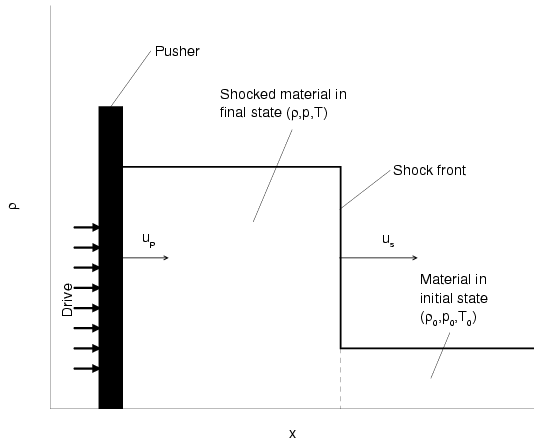
Shock wave experiments are an established technique (Zeldovich and Raizer, 1966) to
determine the equation of state at high pressures and temperature,
which has been applied to a wide range of materials including
aluminum, iron, and water. In the experiment, a driving force is
utilized to propel a pusher at constant velocity ![]() into a material
at predetermined initial conditions (
into a material
at predetermined initial conditions (
![]() ) as shown in
Fig.
) as shown in
Fig. ![[*]](crossref.png) . The impact generates a planar shock wave, which
travels at the constant velocity
. The impact generates a planar shock wave, which
travels at the constant velocity ![]() with
with ![]() . The shock
compression drives the material to a point on the principle Hugoniot,
which is the locus of all final states characterized by (
. The shock
compression drives the material to a point on the principle Hugoniot,
which is the locus of all final states characterized by (![]() )
that can be achieved by a single shock wave passing through. Under the
assumption of an ideal shock (see below), the conservation laws of
mass, momentum, and energy require only the measurement of the
velocities of the pusher
)
that can be achieved by a single shock wave passing through. Under the
assumption of an ideal shock (see below), the conservation laws of
mass, momentum, and energy require only the measurement of the
velocities of the pusher ![]() and the shock front
and the shock front ![]() in order to
obtain an absolute equation of state data point. Pressure and density
of the shock material are related to
in order to
obtain an absolute equation of state data point. Pressure and density
of the shock material are related to ![]() and
and ![]() by,
by,
By an ideal shock, one means that a planar pusher is driven at constant
velocity into the sample. The resulting shock wave is characterized by
a planar shock front that travels at constant velocity during the
measurement. Furthermore, one assumes that unshocked material remains
at known initial conditions and not preheated as for example by x-rays
created at the laser target interaction. Under these assumptions, one
can determine the equation of state from the measured velocities ![]() and
and ![]() using Eqs. -.
using Eqs. -.
![\includegraphics[angle=270,width=10cm]{figures4/graph_hug84_paper1.eps}](graph_hug84_paper1.png) |
In the recent laser shock experiments, a shock wave is propagating
through a sample of pre-compressed liquid deuterium characterized by
an initial state, (![]() ,
,
![]() ,
, ![]() ) with
) with
![]() and
and
![]() . In our calculations, we set
. In our calculations, we set ![]() to
its exact value of
to
its exact value of
![]() per atom (Kolos and Wolniewicz, 1964) and
per atom (Kolos and Wolniewicz, 1964) and ![]() because
because ![]() . Using the PIMC simulation results for
. Using the PIMC simulation results for ![]() and
and
![]() , we calculate
, we calculate ![]() from Eq. and then
interpolate
from Eq. and then
interpolate ![]() linearly at constant
linearly at constant ![]() between the two densities
corresponding to
between the two densities
corresponding to ![]() and
and ![]() to obtain a point on the
Hugoniot in the
to obtain a point on the
Hugoniot in the ![]() plane. Results at
plane. Results at ![]() confirm
that the function is linear within the statistical errors. The PIMC
data for
confirm
that the function is linear within the statistical errors. The PIMC
data for ![]() ,
, ![]() , and the Hugoniot are given in Tab. .
, and the Hugoniot are given in Tab. .
|
|
|
|
|
|||
| 1000000 | 53.79 (5) | 245.7 (3) | 66.85 (8) | 245.3 (4) | 0.7019 (1) | 56.08 (5) |
| 500000 | 25.98 (4) | 113.2 (2) | 32.13 (5) | 111.9 (2) | 0.7130 (1) | 27.48 (4) |
| 250000 | 12.12 (3) | 45.7 (2) | 14.91 (3) | 44.3 (2) | 0.7242 (1) | 12.99 (2) |
| 125000 | 5.29 (4) | 11.5 (2) | 6.66 (2) | 11.0 (1) | 0.7300 (3) | 5.76 (2) |
| 62500 | 2.28 (4) | -3.8 (2) | 2.99 (4) | -3.8 (2) | 0.733 (1) |
2.54 (3) |
| 31250 | 1.11 (6) | -9.9 (3) | 1.58 (7) | -9.7 (3) | 0.733 (3) |
1.28 (5) |
| 15625 | 0.54 (5) | -12.9 (3) | 1.01 (5) | -12.0 (2) | 0.721 (4) |
0.68 (4) |
| 10000 | 0.47 (5) | -13.6 (3) | 0.80 (8) | -13.2 (4) | 0.690 (7) |
0.51 (5) |
In Fig. , we compare the effects of different
approximations made in the PIMC simulations such as time step ![]() ,
number of pairs
,
number of pairs ![]() and the type of nodal restriction. For pressures
above 3 Mbar, all these approximations have a very small effect. The
reason is that PIMC simulation become increasingly accurate as
temperature increases. The first noticeable difference occurs at
and the type of nodal restriction. For pressures
above 3 Mbar, all these approximations have a very small effect. The
reason is that PIMC simulation become increasingly accurate as
temperature increases. The first noticeable difference occurs at
![]() , which corresponds to
, which corresponds to
![]() . At
lower pressures, the differences become more and more pronounced. We
have performed simulations with free particle nodes and
. At
lower pressures, the differences become more and more pronounced. We
have performed simulations with free particle nodes and ![]() for
three different values of
for
three different values of ![]() . Using a smaller time step makes the
simulations computationally more demanding and it shifts the Hugoniot
curves to lower densities. These differences come mainly from
enforcing the nodal surfaces more accurately, which seems to be more
relevant than the simultaneous improvements in the accuracy of the
action
. Using a smaller time step makes the
simulations computationally more demanding and it shifts the Hugoniot
curves to lower densities. These differences come mainly from
enforcing the nodal surfaces more accurately, which seems to be more
relevant than the simultaneous improvements in the accuracy of the
action ![]() , that is the time step is more constrained by the Fermi
statistics than it is by the potential energy. We improved the
efficiency of the algorithm by using a smaller time step
, that is the time step is more constrained by the Fermi
statistics than it is by the potential energy. We improved the
efficiency of the algorithm by using a smaller time step ![]() for
evaluating the Fermi action than the time step
for
evaluating the Fermi action than the time step ![]() used for the
potential action. Unless specified otherwise, we used
used for the
potential action. Unless specified otherwise, we used
![]() . At even lower pressures not shown in Fig.
, all of the Hugoniot curves with FP nodes
turn around and go to low densities as expected.
. At even lower pressures not shown in Fig.
, all of the Hugoniot curves with FP nodes
turn around and go to low densities as expected.
As a next step, we replaced the FP nodes by VDM nodes. Those results
show that the form of the nodes has a significant effect for ![]() below
2 Mbar. Using a smaller
below
2 Mbar. Using a smaller ![]() also shifts the curve to slightly lower
densities. In the region where atoms and molecules are forming, it is
plausible that VDM nodes are more accurate than free nodes because
they can describe those states (see
chapter 3). We also
show a Hugoniot derived on the basis of the VDM alone (dashed line).
These results are quite reasonable considering the approximations
(Hartree-Fock) made in that calculation. Therefore, we consider the
PIMC simulation with the smallest time step using VDM nodes
(
also shifts the curve to slightly lower
densities. In the region where atoms and molecules are forming, it is
plausible that VDM nodes are more accurate than free nodes because
they can describe those states (see
chapter 3). We also
show a Hugoniot derived on the basis of the VDM alone (dashed line).
These results are quite reasonable considering the approximations
(Hartree-Fock) made in that calculation. Therefore, we consider the
PIMC simulation with the smallest time step using VDM nodes
(![]() ) to be our most reliable Hugoniot. Going to bigger system
sizes
) to be our most reliable Hugoniot. Going to bigger system
sizes ![]() and using FP nodes also shows a shift towards lower
densities.
and using FP nodes also shows a shift towards lower
densities.
|
|
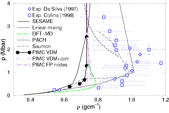
Fig. compares the Hugoniot from laser shock wave
experiments (Da Silva, 1997; Collins et al., 1998) with PIMC simulations (VDM nodes,
![]() ) and several theoretical approaches:
SESAME model by Kerley (1983) (thin solid line), linear mixing model
(dashed line) by Ross (1998), DFT-MD by Lenosky et al. (2000) (dash-dotted
line), Padé approximation in the chemical picture (PACH) by
Ebeling and Richert (1985a) (dotted line), and the work by Saumon and Chabrier (1992) (thin
dash-dotted line).
) and several theoretical approaches:
SESAME model by Kerley (1983) (thin solid line), linear mixing model
(dashed line) by Ross (1998), DFT-MD by Lenosky et al. (2000) (dash-dotted
line), Padé approximation in the chemical picture (PACH) by
Ebeling and Richert (1985a) (dotted line), and the work by Saumon and Chabrier (1992) (thin
dash-dotted line).
|
The differences of the various PIMC curves in
Fig. as well as in Fig.
are small compared to the deviation from the experimental results by
Da Silva (1997) and Collins et al. (1998). One finds that the corrections from
Eq. have only a small effect on the Hugoniot. In the
experiments, an increased compressibility with a maximum value of ![]() was found while PIMC predicts
was found while PIMC predicts ![]() , only slightly higher than that given by the SESAME
model. Only for
, only slightly higher than that given by the SESAME
model. Only for
![]() , does our Hugoniot lie within
experimental error bars. In this regime, the deviations in the PIMC
and PACH Hugoniot are relatively small, less than
, does our Hugoniot lie within
experimental error bars. In this regime, the deviations in the PIMC
and PACH Hugoniot are relatively small, less than
![]() in density. In the high pressure limit, the Hugoniot goes to
the FP limit of 4-fold compression. This trend is also present in the
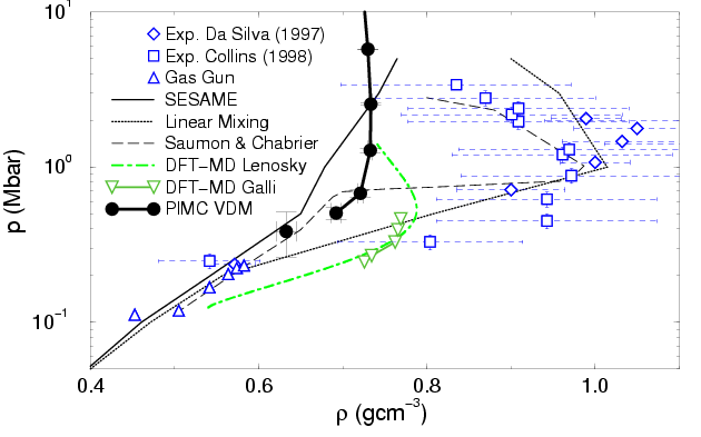
experimental findings. For pressures below 1 Mbar, the PIMC Hugoniot
goes back to lower densities and shows the expected tendency towards the
experimental values from earlier gas gun work
Nellis et al. (1983); Holmes et al. (1995) and lowest data points from Da Silva (1997); Collins et al. (1998).
This trend can be studied best in the logarithmic graph shown in
Fig , where we also included our lowest available
pressure point on the Hugoniot, which was obtained from simulations with 32
pairs of electrons and deuterons and the time step
in density. In the high pressure limit, the Hugoniot goes to
the FP limit of 4-fold compression. This trend is also present in the
experimental findings. For pressures below 1 Mbar, the PIMC Hugoniot
goes back to lower densities and shows the expected tendency towards the
experimental values from earlier gas gun work
Nellis et al. (1983); Holmes et al. (1995) and lowest data points from Da Silva (1997); Collins et al. (1998).
This trend can be studied best in the logarithmic graph shown in
Fig , where we also included our lowest available
pressure point on the Hugoniot, which was obtained from simulations with 32
pairs of electrons and deuterons and the time step
![]() and
and
![]() .
Within the statistical error bars, the PIMC Hugoniot curve tends
towards the results from gas gun experiments. For these low pressures,
one also finds that the differences between PIMC and DFT-MD are also
relatively small compared to the deviation from the laser shock data.
.
Within the statistical error bars, the PIMC Hugoniot curve tends
towards the results from gas gun experiments. For these low pressures,
one also finds that the differences between PIMC and DFT-MD are also
relatively small compared to the deviation from the laser shock data.
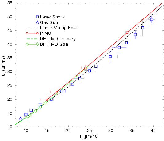
Using the PIMC equation of state, one can also determine the shock and
pusher velocity on the Hugoniot. From Eqs. and
, one finds,
 |
(206) | ||
 |
(207) |
and compared to the
experimental shock and pusher velocities published in
(Collins et al., 1998). First of all, one finds the differences between
theory and experiment are not as pronounced as in the . This fact simply follows from
Eq. where one divides by the difference of . Possibly the experiments allow a more
accurate determination of the difference
Summarizing, one can say that PIMC simulations predict a slightly
increased compressibility of ![]() compared to the SESAME
model but they cannot reproduce the experimental findings of values of
about
compared to the SESAME
model but they cannot reproduce the experimental findings of values of
about ![]() . Further theoretical and experimental work will be
needed to resolve this discrepancy.
. Further theoretical and experimental work will be
needed to resolve this discrepancy.
