


Next: Long Range Action
Up: Pair Density Matrix
Previous: Pair Density Matrix
Contents
Short Range Action
The exact pair density matrix for any interaction potential in
infinite volume can be calculated by the matrix squaring technique by
Storer (1968). This method is applied to the short-range part generated
by the Ewald break-up of the Coulomb potential. Since the potential is
short range the periodicity is irrelevant. First, one factorizes the
density matrix into a center-of-mass term and a term depending on the
relative coordinates. The latter term is equivalent to the density
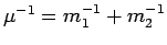
matrix for a particle with the reduced mass
 in an external potential. The one expands the pair density
matrix in partial waves. In
in an external potential. The one expands the pair density
matrix in partial waves. In  dimensions, it reads,
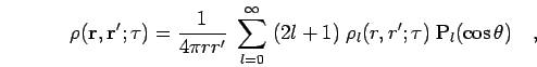 |
(41) |
where  is the angle between
  and
and  and P
and P denotes
the
denotes
the  th Legendre polynomial. For spherically symmetric interaction
potentials, different partial wave components
th Legendre polynomial. For spherically symmetric interaction
potentials, different partial wave components  do not mix and
can be derived from independent matrix squaring procedures. The six
dimensional pair density matrix is reduced to a sum of two dimensional
objects. Each component satisfies a 1 dimensional Bloch
equation with an additional term,
do not mix and
can be derived from independent matrix squaring procedures. The six
dimensional pair density matrix is reduced to a sum of two dimensional
objects. Each component satisfies a 1 dimensional Bloch
equation with an additional term,
![\begin{displaymath}
- \frac{\partial \rho_l(r,r';\beta)}{\partial \beta} =
\lef...
...
\frac{ \lambda}{r^2} \: l(l+1) \: \right] \rho_l(r,r';\beta)
\end{displaymath}](img299.png) |
(42) |
and also fulfills the convolution equation,
 |
(43) |
This is a one dimensional integral for a given pair of  and
and  ,
which can be calculated numerically. In order to derive the pair
density matrix for a time step
,
which can be calculated numerically. In order to derive the pair
density matrix for a time step
 , one typically
performs of the order of
, one typically
performs of the order of  matrix squarings starting at the
inverse temperature
matrix squarings starting at the
inverse temperature
 . The partial
waves are initialized using semi-classical expression analogous to
Eq. 2.29, for details see Ceperley (1995) and Magro (1996). The
resulting pair density matrix can be verified by using the Feynman-Kac
formula Eq. 2.27 in a separate MC simulation (Pollock and Ceperley, 1984).
. The partial
waves are initialized using semi-classical expression analogous to
Eq. 2.29, for details see Ceperley (1995) and Magro (1996). The
resulting pair density matrix can be verified by using the Feynman-Kac
formula Eq. 2.27 in a separate MC simulation (Pollock and Ceperley, 1984).
The pair density matrix is between two particles at initial position
 and final position
 needs to be
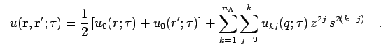
evaluated very frequently in a PIMC simulation. Using the fact that
initial and final position cannot be too far apart, one can expand the
action in a power series. It is convenient to use the three distance
needs to be
evaluated very frequently in a PIMC simulation. Using the fact that
initial and final position cannot be too far apart, one can expand the
action in a power series. It is convenient to use the three distance
where
 and
and
 . The variables
  and
and  are of the order of
 . The action can then be expanded as,
 |
(47) |
where  denotes the order of the expansion. In zeroth order,
only the first term, the end-point action, is considered. The
following terms are off-diagonal contributions, which are
important because they allow to reduce the number of time slices in a
PIMC simulation. The same expansion formula is used for the
contributions to the energy given by
denotes the order of the expansion. In zeroth order,
only the first term, the end-point action, is considered. The
following terms are off-diagonal contributions, which are
important because they allow to reduce the number of time slices in a
PIMC simulation. The same expansion formula is used for the
contributions to the energy given by  derivative of the
action.
derivative of the
action.  denotes the order in this expansion.
Next: Long Range Action
Up: Pair Density Matrix
Previous: Pair Density Matrix
Contents
Burkhard Militzer
2003-01-15
