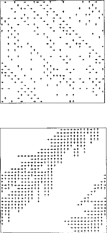
Figure 7: Two configurations of in Bihams two-dimensional cellular automata model by Biham el al. [11], a jam-free phase in the upper figure and congested phases below. The arrows denote the direction of moving cars.
In previous sections, we studied the traffic flow in one dimension.
However, in cities the problem is much more complex. One has to
consider the effect of intersection, traffic lights, coupling of
traffic in different directions, turning cars, etc. Several
two-dimensional models were advanced, which allows to incorporate those
effects to a different extent.
A simple CA model in two dimensions was developed by Biham el al.
[11]. The model is defined on a square lattice with periodic
boundary conditions. Each site can be in three states, it contains a car
moving upwards, a car moving to the right or it is empty. The dynamics is
controlled by traffic lights so that cars can move to the right at odd
time steps and upwards on the even time steps. In one time step, cars can
only move to the next site if this is empty.
The described system exhibits two different regimes. At low densities, one
finds a dynamic phase, where the system self-organizes similar cars along
the diagonal and therefore maximizes the average speed (see Fig.
7). At high densities, all cars are jammed in one big cluster,
which leads to an average velocity of zero.
The two phases are separated by a sharp transition at a critical density,
which is size dependent.

Figure 7: Two configurations of in Bihams two-dimensional
cellular automata model by Biham el al. [11], a jam-free phase in the
upper figure and congested phases below. The arrows denote the direction
of moving cars.
In the model described above, cars can never turn. This possibility
was included in a more advanced model by Cuesta el al. [13, 14].
There,
a parameter ![]() is introduced, which determines the direction cars try to
move. For one half of the cars,
is introduced, which determines the direction cars try to
move. For one half of the cars, ![]() specifies the probability of
trying to move upwards and
specifies the probability of
trying to move upwards and ![]() the probability of trying to move
to the right. For the other half of the cars, the opposite probabilities are
assigned. Setting
the probability of trying to move
to the right. For the other half of the cars, the opposite probabilities are
assigned. Setting ![]() , this reproduces Biham's model. An increased
, this reproduces Biham's model. An increased
![]() gives car the possibility to take advantage of open sites out of their
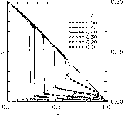
main direction of motion. This flexibility shifts the jamming transition
to a higher density. This is shown in Fig. 8, which can be explained
in terms of a first order transition critical point between
gives car the possibility to take advantage of open sites out of their
main direction of motion. This flexibility shifts the jamming transition
to a higher density. This is shown in Fig. 8, which can be explained
in terms of a first order transition critical point between
![]() .
.

Figure 8: Average velocity versus car density at different randomness
value ![]() by Cuesta el al. [13]
by Cuesta el al. [13]
In a following paper [14], the same system was studied using a non-linear
Boltzmann equation. This approach can predict the existence of the jamming
transition and physical quantities but does not show the correct ![]() dependence.
dependence.
A much more elaborate model with realistic traffic rules
was given by Freund el al. [12].
In this model, a city is represented by
L vertical and horizontal two-way streets, which leads to ![]() crossing.
At each crossing, cars can line up forming queues in every direction
with a maximum length Q. There are no traffic lights but cars follow
the left-before-right traffic rule, which is standard in many countries
(for details see [12]). Each time a car lines up at a crossing
the desired direction is chosen at random. A car can only cross an intersection
if it has the right of way and the desired street is not fully occupied.
crossing.
At each crossing, cars can line up forming queues in every direction
with a maximum length Q. There are no traffic lights but cars follow
the left-before-right traffic rule, which is standard in many countries
(for details see [12]). Each time a car lines up at a crossing
the desired direction is chosen at random. A car can only cross an intersection
if it has the right of way and the desired street is not fully occupied.
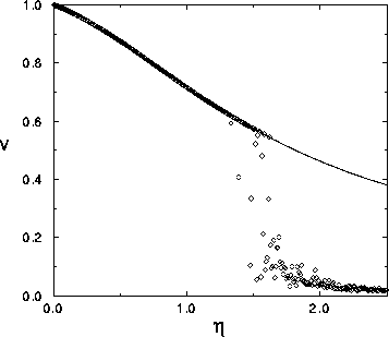
Numerical studies in [12] show a sharp jamming transition near
a critical car density of ![]() (Fig. 9).
Above this density, one still finds a remanent average velocity,
which indicates that some jams may dissolve under those rules.
(Fig. 9).
Above this density, one still finds a remanent average velocity,
which indicates that some jams may dissolve under those rules.

Figure 9: Average velocity versus density from simulation (![]() ) and
statistical methods (solid line) by Freund el al. [12]
) and
statistical methods (solid line) by Freund el al. [12]
The numerical results were compared to predictions from statistical theory, in which the two-dimensional flow was described by a Bernoulli-process. The agreement is remarkably good until the jamming transition occurs (see Fig. 9).