An overview of the field is given in the work by Prigogine el al. [1] on kinetic theory of vehicular traffic. The traffic flow can be understood by studying the distribution function f(x,v,t), which describes the number of cars in the road interval (x,x+dx) with a velocity in (v,v+dv) at a given time t. A few measurements have been made to determine this function (see Fig. 1).
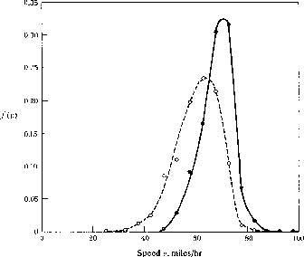
Figure 1: Measured velocity distribution function f(v) versus velocity v.
(taken from [1]).
This function can also be expressed in terms of the two fundamental variables, concentration and flow (or current). An understanding of the relation of concentration and flow is the basis for describing the traffic. The flow-concentration curve is called the fundamental diagram of road traffic or the equation of state of traffic theory. Two measurements of this function are shown in Fig. 2.
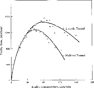
Figure 2: Fundamental diagram: Flow versus vehicle concentration is shown
in this fundamental diagram
for two different tunnels.
(taken from [1]).
At low densities, the flow increases linearly with concentration. Cars move independently in the dilute traffic with small fluctuations about a mean velocity. With increasing concentration, cars hinder each other more and more, which leads to a reduction of the average velocity and a decreasing slope in the fundamental diagram. These hindering effects become dominant at high concentrations. At a critical density, the flow exhibits a maximum. Then, an increase in density results into an actual decrease of the total throughput, and finally in a completely congested phase where no car can move and the flow is zero.
The flow near the critical concentration is unstable. Small perturbations
that increase the density locally lead to a decrease in the flow,
which then amplifies the initial perturbation. The
variance in car velocities
is what triggers this process [6], which leads to the
formation of traffic jams. Traffic jams are locally congested phases, in which
cars travel at slow or zero velocity. Between jams, one finds cars
at low concentrations traveling with high velocities. These congested phases
are rather stable configurations with their own dynamics. Cars driving into
the jams stabilize and cars leaving from the front can reduce the length.
From this picture, it follows that jams move slowly in the opposite
direction of the cars.
Their velocity can be estimated in a very simple model where one
assumes a small constant velocity ![]() and a density
and a density ![]() in the jam and a higher velocity
in the jam and a higher velocity ![]() and low density
and low density ![]() outside.
If cars accelerate and decelerate instantly, the jam moves with a velocity,
outside.
If cars accelerate and decelerate instantly, the jam moves with a velocity,
![]()
Since the density ratio is small, jams move slowly.
A much more sophisticated picture of jams is given by the theory of fluid
dynamics, in which jams are modeled in terms of density waves.