Next: Variational Density Matrix Properties
Up: Variational Density Matrix Technique
Previous: Analogy to Real-Time Wave
Contents
As a first example, we apply this method to the problem of one particle
in an external potential
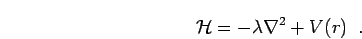 |
(144) |
The one-particle density matrix will be
approximated as a Gaussian with mean  , width
  and
amplitude factor
and
amplitude factor  ,
,
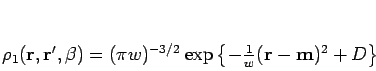 |
(145) |
as variational parameters.
The initial conditions at
 are
are
 ,
,
 and
and  in order to regain the correct free particle limit, Eq. 3.23.
For this ansatz
in order to regain the correct free particle limit, Eq. 3.23.
For this ansatz  , defined in Eq. 3.20 as
![\begin{displaymath}
H\equiv\int \rho{\mathcal{H}}\rho\;{\bf d}{\bf r}=
\left( \frac{3\lambda}{w}+V^{[0]} \right)
\frac{e^{2D}}{(2\pi w)^{3/2}}
\end{displaymath}](img598.png) |
(146) |
where
![\begin{displaymath}
V^{[n]}\equiv \left({2\over \pi w}\right)^{3/2}\int ({\bf r}-{\bf m})^{n} V(r)
e^{-2({\bf r}-{\bf m})^{2}/w} {\bf d}{\bf r}
\end{displaymath}](img599.png) |
(147) |
and
![\begin{displaymath}
N\equiv \int \rho \rho' {\bf d}{\bf r}=
[\pi (w+w')]^{-3/2}
...
...left\{-({\bf m}-{\bf m}')^{2}/(w+w')\right\}\exp( D+D') \quad.
\end{displaymath}](img600.png) |
(148) |
From Eq. 3.19, the equations for the variational
parameters are,
In absence of a potential, the exact free particle density matrix is recovered.
The harmonic oscillator case is also correct since the Gaussian
approximation is exact there.
For a hydrogen atom,  ,
, 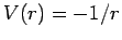 and
and
At low temperature, the density matrix as a function of  goes to the ground state
wave function as discussed in more detail in the next section.
One expects this to be a fixed
point of the dynamics of the parameters and determined by
goes to the ground state
wave function as discussed in more detail in the next section.
One expects this to be a fixed
point of the dynamics of the parameters and determined by
 and
and  while
while  .
The
.
The
 fixed point:
  ,
,  ,
,
 corresponds to the well known Rayleigh-Ritz variational result
for a Gaussian trial wave function
corresponds to the well known Rayleigh-Ritz variational result
for a Gaussian trial wave function
 |
(155) |
In ground state variational studies, addition of two more Gaussians
brings the ground state energy to within  % of the exact value
and similar improvement would be obtained here.
% of the exact value
and similar improvement would be obtained here.
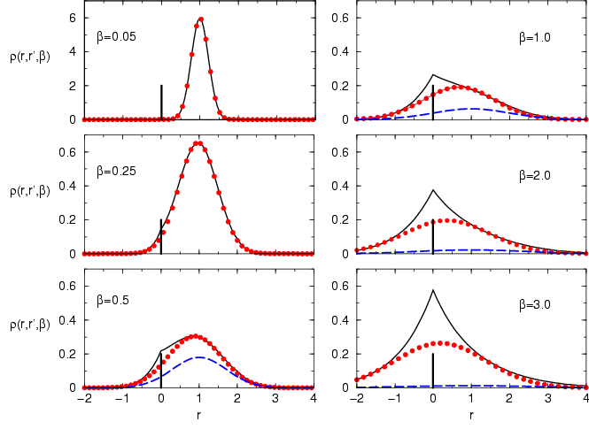
Results at finite  require a numerical solution, which is
illustrated in the figure below comparing the Gaussian variational density matrix
with the exact (Pollock, 1988) and the free particle density matrix at several temperatures
for the initial condition
require a numerical solution, which is
illustrated in the figure below comparing the Gaussian variational density matrix
with the exact (Pollock, 1988) and the free particle density matrix at several temperatures
for the initial condition  . At high temperatures
(
. At high temperatures
( and
and  )
the Gaussian approximation correctly reproduces the limiting free particle
density matrix. At lower temperatures, the cusp in the exact density matrix
due to the Coulombic singularity at the proton becomes evident and
the peak shifts to the origin somewhat faster than the Gaussian variational
approximation. As increases the exact result grows faster than
the variational since the correct energy,
)
the Gaussian approximation correctly reproduces the limiting free particle
density matrix. At lower temperatures, the cusp in the exact density matrix
due to the Coulombic singularity at the proton becomes evident and
the peak shifts to the origin somewhat faster than the Gaussian variational
approximation. As increases the exact result grows faster than
the variational since the correct energy,  , is lower than
  but
the Gaussian variational approximation remains rather accurate for
but
the Gaussian variational approximation remains rather accurate for  .
The free particle density matrix remains centered at
.
The free particle density matrix remains centered at  and
beyond
and
beyond  (
( eV) bears little resemblance to the
correct result.
eV) bears little resemblance to the
correct result.
Figure 3.1:
Comparison of the Gaussian variational approximation (circles)
with the exact density matrix
 (solid line)
for a hydrogen atom. The free particle density matrix (dashed line)
is also shown. The plotted
(solid line)
for a hydrogen atom. The free particle density matrix (dashed line)
is also shown. The plotted  is along the line from the proton at
the origin (marked by the vertical bar) through the initial electron
position
is along the line from the proton at
the origin (marked by the vertical bar) through the initial electron
position  .
.
|
|
Next: Variational Density Matrix Properties
Up: Variational Density Matrix Technique
Previous: Analogy to Real-Time Wave
Contents
Burkhard Militzer
2003-01-15
![$\displaystyle 4 \lambda + 2 w V^{[0]} - \frac{8}{3} V^{[2]}$](img602.png)
![$\displaystyle \frac{1}{2} V^{[0]} - \frac{2}{w} V^{[2]}\quad\;.$](img606.png)
![$\displaystyle {{\bf m}\over m^3}{w\over 4}\left[ \mbox{erf}\left(m\sqrt{2/w}\right)-
\sqrt{8\over \pi w}e^{-2m^2/w}\right ]$](img612.png)
![$\displaystyle \sqrt{w\over 2\pi}e^{-2m^2/w}+
{3 w\over 4}V^{[0]}\quad.$](img614.png)