Example: One Hydrogen Atom

The off-diagonal sampling procedure can be simplified for the application to the electronic excitations in hydrogen. For all temperatures under consideration, the thermal de Broglie wave length of the protons is small compared to the inter-particle spacing and also much smaller than that of the electrons. Therefore, one can make the protons classical within a first approximation. In this case, one replaces the proton path by a point particle and needs only one open electron path. The pairs ${\bf r}$ and ${\bf r}'$ in Eq. 5.15 are then given by the separation of the ends of the electron paths and the proton. This has the advantage that one can average over all protons in a many proton simulation discussed in section 5.4.3.

Figure 5.9: Natural orbitals (solid lines) $\frac{1}{r}\phi_{li}(r) \equiv R_{nl}(r)$ with $n=l+i$ for a single hydrogen atom in a periodically repeated box of size $L=10.2$, which were generated from a simulation at $T=250\,000\,\rm K$. The columns correspond to the eigenvectors with angular momentum $l$ calculated by diagonalizing the matrix $\rho _l(r,r')$. The rows show the $i$th eigenvector beginning with the highest eigenvalue corresponding to lowest energy state. For $n \leq 3$ the eigenstates of the isolated hydrogen atom are shown as dash-dotted lines. The isolated 1s state is almost identical to the corresponding natural orbit and is therefore hidden behind the other line.

In the PIMC simulation, one calculates the matrices for a certain number of angular momentum states using the average given by Eq. 5.16. We kept the matrices for $l\leq 5$ and used a uniform grid in real space with 50 points from $r=0$ to $L/2\sqrt{3}$. This includes an approximation because one does not consider the cubic symmetry of the simulation cell. In the limit of a large cell, this approximation becomes more and more accurate because the majority of the occupied natural orbitals only extends over a fraction of the simulation cell and therefore is not affected by the boundary conditions. The justification for using this basis is that one is generally interested in systems where the natural orbitals are determined by the interactions rather than by boundary effects. However, in systems where those are important, another basis that includes the cubic symmetry is more appropriate. Suggestions have been made by Shumway (1999).

The resulting matrices $\rho^{[2]}_l(r,r')$ are then diagonalized, which leads to natural orbitals as eigenvectors and eigenvalues proportional to the occupation numbers. The relative occupation numbers $n_{li}$ are obtained by dividing the eigenvalues by the sum of the traces of all $l$ matrices. We found that the contributions from different matrices decay rapidly with $l$ and that keeping matrices for $l\leq 5$ is more than sufficient.

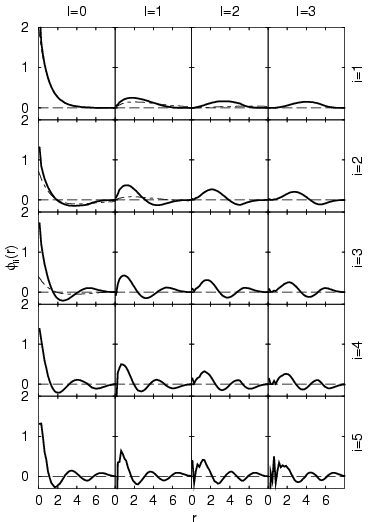
The resulting natural orbitals for a single hydrogen atom in a periodically repeated box of size $L=10.2$ are shown in Fig. 5.9. The displayed functions $\frac{1}{r}\phi_{li}(r)$ are expected to approach the radial part $R_{nl}(r)$ with $n=i+l$ of the isolated hydrogen atom in the limit of a large box size. The example reveals a ground state that is identical within statistical and grid errors to the 1s ground state of the isolated hydrogen atom. Studying the eigenvectors at any $l$ with increasing excitations $i$, one finds that one additional node is introduced at each step $i$. The states with $n=l+i>1$ are similar but not identical to those of the isolated hydrogen atom because the finite size of the simulation cell $L/2=5.1$ does have an effect, which leads to more localized eigenstates. One also notices that the level of numerical noise in the eigenvectors increases with $n$. These effects seems to be the strongest near the origin, which suggests that a different basis such as hydrogen orbitals would lead to a lower noise level. Generally, one finds that the noise in the eigenvectors (using the uniform spatial grid) increases for lower temperatures because the occupation number of higher energy states becomes very small. In this case, the eigenvectors are approximately degenerate ( $n_{li}=n_{l\,i+1}$) and the noise causes that those states are mixed in the diagonalization procedure. This explains why the noise level in the high eigenvectors increase for lower temperature.

Figure 5.10: Cumulative plot of the occupation numbers for the 6 lowest eigenstates (see Fig. 5.9) of a single hydrogen atom in a periodically repeated box of size $L=10.2$ shown as a function of temperature.

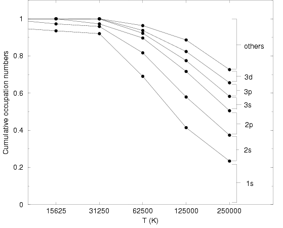Studying the eigenvalues, one finds that there are a few large positive ones while many others are small and some even negative. The occupation numbers are shown in Fig. 5.10 as a function of temperature. One finds that the occupation probability of the 1s ground state increases with decreasing $T$. Within the noise level of about 4%, it goes to 1 in the limit of low $T$. Furthermore, one finds that the occupation of the 2s and 2p are almost the same despite the fact that the 2 eigenvalues come from different matrices. The same argument holds for the 3s, 3p, and 3d level. One can also calculate the differences in energy from the ratio of the occupation numbers. For $E_{\rm 2s}-E_{\rm 1s}$, one finds $9.2\,\rm eV$ rather than $10.2\,\rm eV$ as expected for the isolated hydrogen atom. These deviations increase if higher levels are studied because higher states are more delocalized and therefore increasingly altered by the boundary effects.