Overview
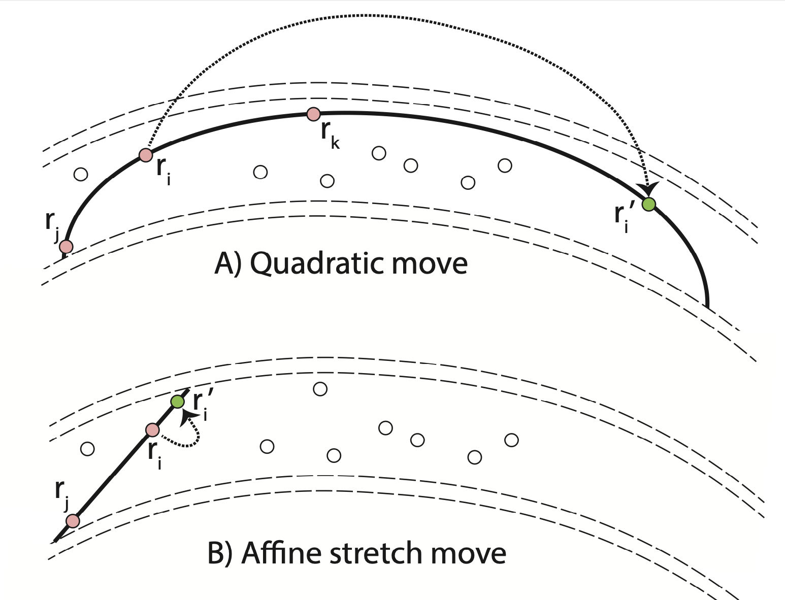
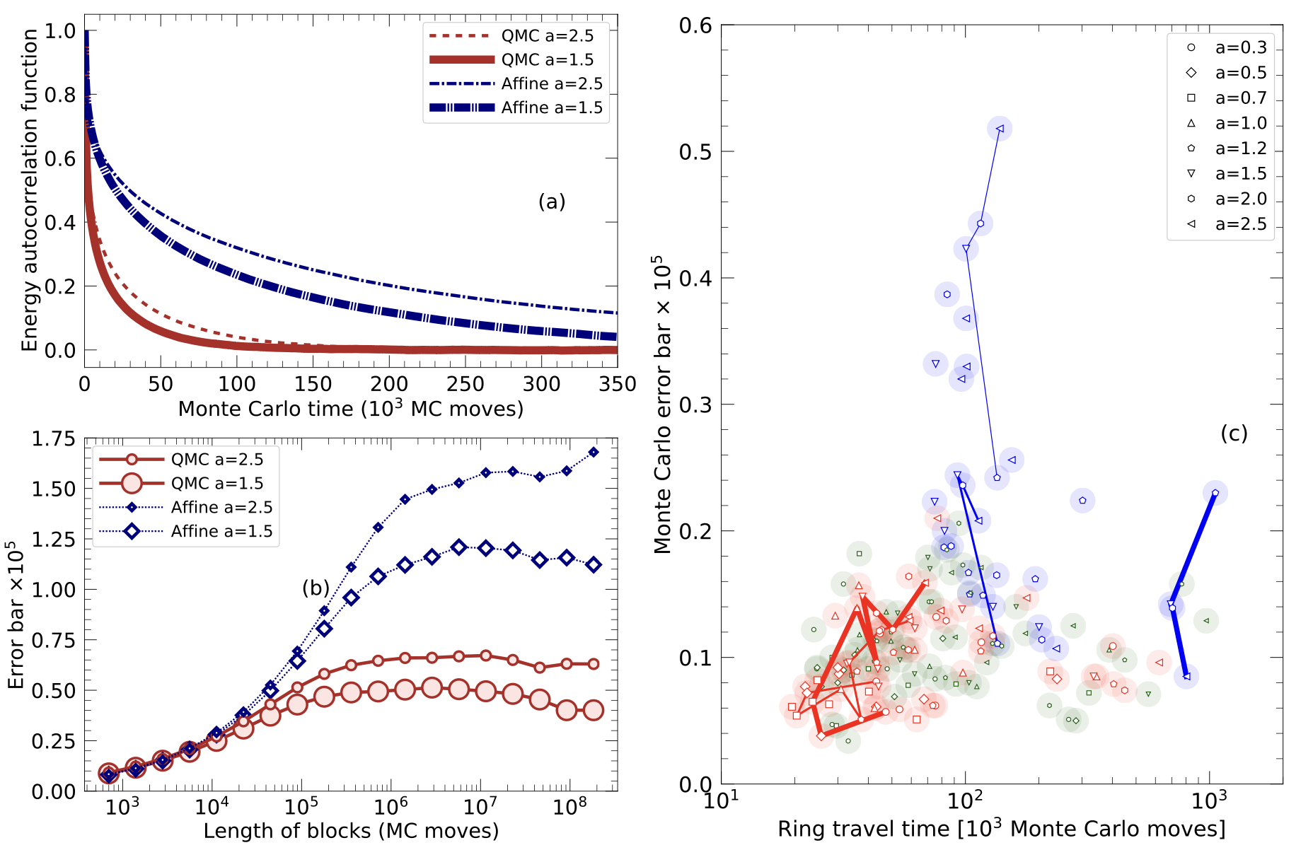
We introduce a new general-purpose Quadratic Monte Carlo (QMC) technique that is more efficient in confining fitness landscapes than the affine-invariant method that relies on linear stretch moves. We compare how long it takes the ensembles of walkers in both methods to travel to the most relevant parameter region. Once there, we compare the autocorrelation time and error bars of the two methods. For a ring potential and the 2D Rosenbrock function, we find that our quadratic Monte Carlo technique is significantly more efficient. Furthermore, we modified the walk moves by adding a scaling factor.
Below we provide the C++ source code and examples so that this method can be applied elsewhere.
Recommended citation: B. Militzer, “ Study of Jupiter's Interior with Quadratic Monte Carlo Simulations”, Astrophysical Journal 953 (2023) 111.
(1) Download the latest version
Our code also has a DOI: 10.5281/zenodo.8038144
| Date | File description | Download link |
|---|---|---|
| We report five novel ensemble Monte Carlo moves in a new manuscript that was accepted for publication in Comp. Phys. Comm. Our updated source code was uploaded to Zenodo and is available here: | qmc_08-10-23.tar.gz | |
| Code submitted along with accepted version of our manuscript. We added code to sample the 2D Rosenbrock function. | qmc_03-08-23.tar.gz | |
| Submitted along with initial manuscript submission to ApJ. | qmc_07-03-22.tar.gz |
(2) License
Our code is currently distributed under the Creative Commons Attribution 4.0 International (CC BY 4.0) license.
(3) Installation
To install our QMC code, download, ungzip, and untar the latest version, change into the QMC directory and run make:
machine:~/QMC_source_code_03-08-23> make
g++ -O3 -Wall -pedantic -funroll-loops  -DRING       Standard.C Main.C Form.C Timer.C PrintErrorBar.C  -lm -o ring
g++ -O3 -Wall -pedantic -funroll-loops  -DHARMONIC   Standard.C Main.C Form.C Timer.C PrintErrorBar.C  -lm -o harm
g++ -O3 -Wall -pedantic -funroll-loops  -DROSENBROCK Standard.C Main.C Form.C Timer.C PrintErrorBar.C  -lm -o rosen
This invokes the GNU C++ compiler g++ with -O3 for optimization. The arguments -Wall -pedantic -funroll-loops are optional. It generates three executables—ring, harm, and rosen—to sample our ring potential, a harmonic potential, and the 2D Rosenbrock density, respectively. For details please read our manuscript in ApJ.
If compilation fails, try editing the Makefile or switch to a different compiler. We do not provide executables for any operating system here, but our source code has compiled successfully with:
- Linux
g++version 4.8.4 (Ubuntu 4.8.4-2ubuntu1~14.04.4) - Linux
g++version 4.8.5 (Red Hat 4.8.5-44) (GCC) - macOS
clangversion 14.0.3 (clang-1403.0.22.14.1) - Intel
icpcversion 2021.6.0
To compile and run our code, you need a C++ compiler. On macOS, we recommend installing Xcode with the command-line tools. On Windows, please install Cygwin with g++ version 10.2.1 or later.
(4) Included files
The most important lines of code are in MC.h and Main.C. To understand the implementation of the QMC method, we recommend opening MC.h and reading the function PerformOneQuadraticMonteCarloSweep(...). The most relevant lines of code are shown here in simplified form:
Array1 <S> s = SetUpNStates(nWalkers);           // Set up nWalkers different states of type S
for (int iBlock = 0; iBlock < nBlocks; iBlock++) {         // loop over blocks
  for (int iStep = 0; iStep < nStepsPerBlock; iStep++) {   // loop over steps
    for (int i = 0; i < nWalkers; i++) {                   // try moving every walker once per step
      int j, k;
      SelectTwoOtherWalkersAtRandom(i, j, k);

      const double tj = -1.0;
      const double tk = +1.0;
      const double ti   = SampleT(a); // sample t space
      const double tNew = SampleT(a); // sample t space one more time

      const double wi = LagrangeInterpolation(tNew, ti, tj, tk);
      const double wj = LagrangeInterpolation(tNew, tj, tk, ti);
      const double wk = LagrangeInterpolation(tNew, tk, ti, tj);

      S sNew = s[0]; // Create new state by copying an existing one.
      for (int d = 0; d < nDim; d++) {
        sNew[d] = wi * s[i][d] + wj * s[j][d] + wk * s[k][d]; // set nDim parameters of new state
      }

      if (sNew.Valid()) {                 // check if state sNew is valid before calling Evaluate()
        sNew.Evaluate();                  // Sets the energy sNew.y which defines the state's probability = exp(-y/temp)
        double dy   = sNew.y - s[i].y;    // difference in energy between new and old state
        double prob = pow(fabs(wi), nDim) * exp(-dy / temp);   // Note |wi|^nDim and Boltzmann factors
        bool accept = (prob > Random());  // Random() returns a single random number between 0 and 1.

        if (accept) {
          for (int d = 0; d < nDim; d++) {
            s[i][d] = sNew[d]; // copy over state sNew
          }
          s[i].y = sNew.y;      // copy also its energy
        }
      }
    }
    ComputeDifferentEnsembleAverages(s);
  }
  PrintEndOfBlockStatement();
}
PrintEndOfRunStatement();
(5) Execution: Test of harmonic potential (tcsh)
set index = 58
set T = 0.01
set n = 6
set a = 1.5
harm -affine           n=$n a=$a T=${T} nBlocks=100000 > affine${index}_${T}_${n}_${a}.txt &

harm -qmc              n=$n a=$a T=${T} nBlocks=100000 > qmcLin${index}_${T}_${n}_${a}.txt &

harm -qmc    -Gaussian n=$n a=$a T=${T} nBlocks=100000 > qmcGau${index}_${T}_${n}_${a}.txt &

# Compare the output with the following results. The MC average of energy, E, should be close to 0.5*n*T = 0.03

grep "Fraction= 0.9" *58_*.txt
affine58_0.01_6_1.5.txt: Fraction= 0.9 n=  90000 E=     0.03000173 +-     0.00001369
qmcGau58_0.01_6_1.5.txt: Fraction= 0.9 n=  90000 E=     0.03003602 +-     0.00001169
qmcLin58_0.01_6_1.5.txt: Fraction= 0.9 n=  90000 E=     0.02999435 +-     0.00001152
(6) Execution: Ring potential (tcsh)
machine:~/QMC_source_code_03-08-23> tcsh
set index = 57
set T = 0.01
set n = 6
set a = 1.5
set m = 6
set R = 1.0
ring -low -affine           m=$m n=$n a=$a T=${T} R=${R} nBlocks=100000 > affine${index}_${T}_${n}_${m}_${a}_${R}.txt &
ring -low -qmc              m=$m n=$n a=$a T=${T} R=${R} nBlocks=100000 > qmcLin${index}_${T}_${n}_${m}_${a}_${R}.txt &
ring -low -qmc    -Gaussian m=$m n=$n a=$a T=${T} R=${R} nBlocks=100000 > qmcGau${index}_${T}_${n}_${m}_${a}_${R}.txt &

# Compare the output with the following. The MC averages will not agree perfectly.

machine:~/QMC_source_code_03-08-23> grep "Fraction= 0.9" *57_*.txt
affine57_0.01_6_6_1.5_1.0.txt: Fraction= 0.9 n=  90000 E=    -0.00031481 +-     0.00007970
qmcGau57_0.01_6_6_1.5_1.0.txt: Fraction= 0.9 n=  90000 E=    -0.00030795 +-     0.00004486
qmcLin57_0.01_6_6_1.5_1.0.txt: Fraction= 0.9 n=  90000 E=    -0.00026504 +-     0.00003554
(7) Execution: Performance of modified walk moves (Rosenbrock)
machine:~/CMS_MC_test_03-08-23a> tcsh
set index = 199
set T = 1.0
foreach nWalkers (3 4 5 6 8 10 20)
  set para = "T=$T nStepsPerBlock=1000 nBlocks=100000 nWalkers=${nWalkers}"
  foreach nMovers (3 4 5 6 10)
    foreach a (1.2 1.5 2.0 3.0)
      rosen -walk $para nMovers=$nMovers a=$a > walk${index}_${nWalkers}_${nMovers}_${a}.txt &
    end
  end
end
(8) Concluding remarks
At the moment, we do not have a Python version of our QMC code, but it is high on our to-do list.
If you have feedback, comments, or a specific scientific problem you would like to solve, please send email to militzer [at] berkeley [dot] edu.
Best wishes and happy QMC computation!